Build a Large Language Model (From Scratch) Reading Note

Chapter 1

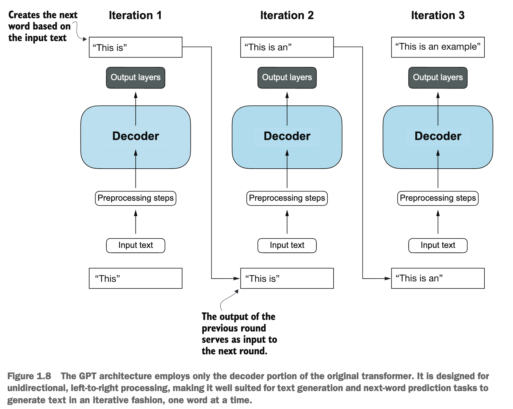
GPT是自回归模型：像GPT这样的解码器式模型，它们生成文本的方式是一次预测一个词 (one word at a time)。也就是说，它会根据已经生成的词语序列来预测下一个最可能出现的词语，然后将这个预测到的词语加入到序列中，再进行下一步的预测，如此循环。这种依赖于自身先前输出进行下一步预测的特性，使得这类模型被称为“自回归模型”（Autoregressive model）。

Chapter 2

Word2Vec trained neural network architecture to generate word embeddings by predicting the context of a word given the target word or vice versa. The main idea behind Word2Vec is that words that appear in similar contexts tend to have similar meanings.

LLMs commonly produce their own embeddings that are part of the input layer and are updated during training. The advantage of optimizing the embeddings as part of the LLM training instead of using Word2Vec is that the embeddings are optimized to the specific task and data at hand.

Tokenizing text

The algorithm underlying BPE breaks down words that aren’t in its predefined vocabulary into smaller subword units or even individual characters, enabling it to handle out-of-vocabulary words.

有三个关键参数：

• 1：每次目标序列都在输入序列的位置上偏移 1 个 Token
• max_length：定义了每个训练样本中输入序列的长度和目标序列的长度
• stride：定义了滑动窗口在 token_ids 上移动的步长

Embedding

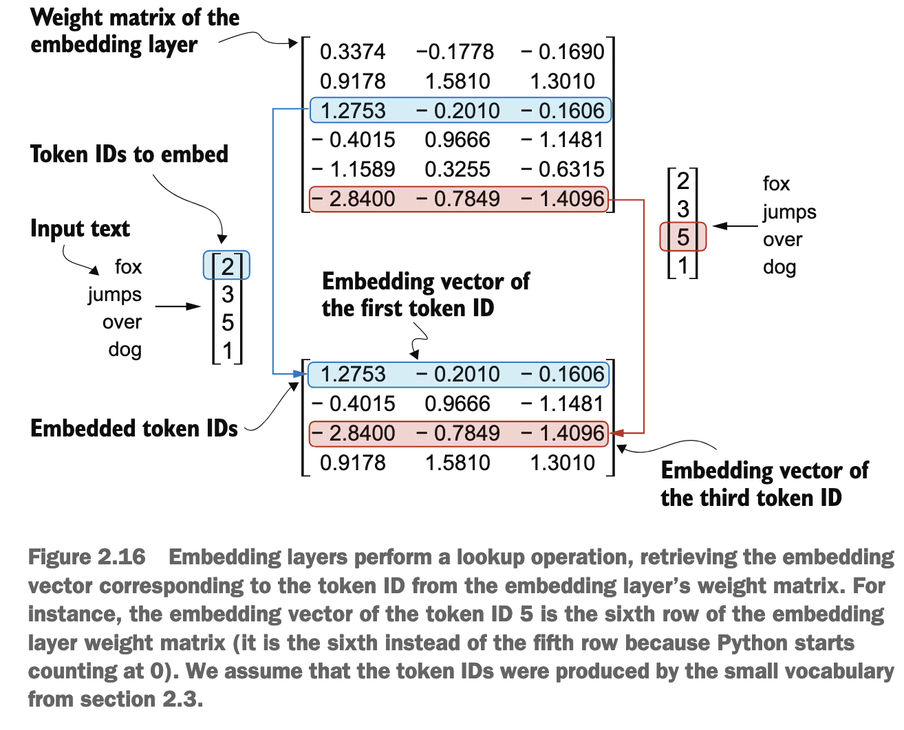
Embedding: TokenId -> Vector

总共几个词汇, embedding layer 就有几个 row, column 数量即为 dimension

In other words, the embedding layer is essentially a lookup operation that retrieves rows from the embedding layer’s weight matrix via a token ID.

The way the previously introduced embedding layer works is that the same token ID always gets mapped to the same vector representation, regardless of where the token ID is positioned in the input sequence.

However, since the self-attention mechanism of LLMs itself is also position-agnostic, it is helpful to inject additional position information into the LLM.

Chapter 3

The big limitation of encoder–decoder RNNs is that the RNN can’t directly access earlier hidden states from the encoder during the decoding phase. Consequently, it relies solely on the current hidden state, which encapsulates all relevant information. This can lead to a loss of context, especially in complex sentences where dependencies might span long distances.

In self-attention, the “self” refers to the mechanism’s ability to compute attention weights by relating different positions within a single input sequence. It assesses and learns the relationships and dependencies between various parts of the input itself, such as words in a sentence or pixels in an image. This is in contrast to traditional attention mechanisms, where the focus is on the relationships between elements of two different sequences, such as in sequence-to-sequence models where the attention might be between an input sequence and an output sequence,

A simple self-attention mechanism without trainable weights

The first step of implementing self-attention is to compute the intermediate values ω, referred to as attention scores.

We determine these scores by computing the dot product of the query, x(2), with every other input token

query = inputs[1]
attn_scores_2 = torch.empty(inputs.shape[0])

for i, x_i in enumerate(inputs):
    attn_scores_2[i] = torch.dot(x_i, query)

print(attn_scores_2)

In the next step, as shown, we normalize each of the attention scores we computed previously. The main goal behind the normalization is to obtain attention weights that sum up to 1.

attn_weights_2_tmp = attn_scores_2 / attn_scores_2.sum() print("Attention weights:", attn_weights_2_tmp)
print("Sum:", attn_weights_2_tmp.sum())

# better to use softmax
attn_weights_2 = torch.softmax(attn_scores_2, dim=0)

Calculating the context vector z(2) by multiplying the embedded input tokens, x(i), with the corresponding attention weights and then summing the resulting vectors.

• Attention weights: 某个 token 与这句话中的其他 token 向量表示的点积, 点积越大, 表明两个向量越相似
• Context vector: 把 attention weight 与对应的 token 的向量相乘, 最后累加

query = inputs[1]
context_vec_2 = torch.zeros(query.shape)
for i,x_i in enumerate(inputs): 
 context_vec_2 += attn_weights_2[i]*x_i print(context_vec_2)

Computing attention weights for all input tokens

attn_scores = torch.empty(6, 6) 
for i, x_i in enumerate(inputs): 
 for j, x_j in enumerate(inputs): 
  attn_scores[i, j] = torch.dot(x_i, x_j)

# we can simplify it to:
attn_scores = inputs @ inputs.T

attn_weights = torch.softmax(attn_scores, dim=-1)


# 同理, 计算 context_vectors 时, 也可以用矩阵乘法:
all_context_vecs = attn_weights @ inputs

• If attn_scores is a two-dimensional tensor (for example, with a shape of [rows, columns]), it will normalize across the columns so that the values in each row (summing over the column dimension) sum up to 1.

Implementing self-attention with trainable weights

Why query, key, and value?

The terms “key,” “query,” and “value” in the context of attention mechanisms are borrowed from the domain of information retrieval and databases, where similar concepts are used to store, search, and retrieve information.

A query is analogous to a search query in a database. It represents the current item (e.g., a word or token in a sentence) the model focuses on or tries to understand. The query is used to probe the other parts of the input sequence to determine how much attention to pay to them.

The key is like a database key used for indexing and searching. In the attention mechanism, each item in the input sequence (e.g., each word in a sentence) has an associated key. These keys are used to match the query.

The value in this context is similar to the value in a key-value pair in a database. It represents the actual content or representation of the input items. Once the model determines which keys (and thus which parts of the input) are most relevant to the query (the current focus item), it retrieves the corresponding values.

Extending single-head attention to multi-head attention

In practical terms, implementing multi-head attention involves creating multiple instances of the self-attention mechanism, each with its own weights, and then combining their outputs.

For multi-head attention with two heads, we obtain:

• Two weight matrices
• Two attention weight metrics
• Two sets of context vectors

The main idea behind multi-head attention is to run the attention mechanism multiple times (in parallel) with different, learned linear projections—the results of multiplying the input data (like the query, key, and value vectors in attention mechanisms) by a weight matrix.

Chapter 4

The main idea behind layer normalization is to adjust the activations (outputs) of a neural network layer to have a mean of 0 and a variance of 1, also known as unit variance.

通过一个数学变换，使得这组激活值的统计特性变为：它们的平均值大约是0，它们的离散程度（方差）大约是 1

这样可以稳定训练过程：通过将每层（对每个样本而言）的输出维持在一个相似的尺度（均值0，方差1），可以使得梯度在网络中传播时更加稳定，减少梯度消失或梯度爆炸的风险

深度学习中的 “shortcut connections”（快捷连接），也经常被称为 “skip connections”（跳跃连接），是一种神经网络的架构设计。

它的核心思想是：允许一部分输入信息（或较浅层网络的特征）直接“跳过”中间的一些层，与更深层网络的输出进行结合。

你可以把它想象成在神经网络的常规层级结构（信息逐层传递）之外，开辟了一些“高速公路”或“捷径”，让信息可以更快、更直接地从网络的早期阶段传递到后期阶段。

它们是如何工作的？

最常见的实现方式是将某一层（或某个模块）的输入 x 直接加到该层（或模块）的输出 F(x) 上。所以，新的输出 H(x) 就变成了：

H(x)=F(x)+x

这里的 F(x) 代表了中间一层或多层网络所做的非线性变换。x 就是那个被“跳过”或“快捷连接”过来的原始输入。

• 如果 x 和 F(x) 的维度不匹配，可能还需要对 x 进行一个线性投影（比如通过一个1x1的卷积或者全连接层）来匹配维度，然后再相加。

为什么使用 Shortcut Connections？它们有什么好处？

1. 解决梯度消失/爆炸问题：

   在非常深的网络中，梯度在反向传播时逐层相乘，很容易变得非常小（梯度消失）或非常大（梯度爆炸），导致网络难以训练。Shortcut connections 提供了一条更直接的路径，使得梯度可以更容易地从深层传播回浅层，有助于缓解这个问题。因为 H(x) 对 x 的梯度中包含了 ∂x∂x​=1 这一项，保证了至少有一部分梯度能够顺畅回传。

2. 更容易训练非常深的网络：

   著名的 ResNet (Residual Networks) 就是通过引入 shortcut connections（在ResNet中称为“残差连接”）成功训练了非常深（上百甚至上千层）的网络。在没有 shortcut connections 的情况下，简单地堆叠层数，当网络达到一定深度后，性能反而会下降（这被称为“退化问题”，degradation problem），这并非由过拟合导致，而是因为深层网络难以优化。Shortcut connections 使得网络更容易学习“恒等映射”（identity mapping），即如果中间层 F(x) 学到的东西没有用，它可以让 F(x) 趋近于0，那么 H(x)≈x，信息就直接通过 shortcut 传递过去了，至少不会让网络性能变差。

3. 学习残差（Residual Learning）：

   在 ResNet 的情境下，网络层 F(x) 不再需要直接学习一个复杂的潜在映射 H(x)，而是学习输入 x 和期望输出 H(x) 之间的“残差”（residual），即 F(x)=H(x)−x。实践证明，学习残差通常比直接学习完整的映射更容易。

4. 特征重用和信息流动：

   Shortcut connections 允许网络的不同部分访问和重用来自较浅层的特征。这对于某些任务（如图像分割中的 U-Net，它有从编码器到解码器的长跳跃连接）尤其重要，因为浅层特征通常包含更多细节信息，而深层特征则更抽象。

总结来说，Shortcut Connections 使得信息和梯度能够在网络中更顺畅地流动，极大地促进了非常深的神经网络的有效训练和性能提升。它们是现代深度学习架构（如 ResNet、DenseNet、U-Net、Transformer等）中的一个关键组成部分。

class ExampleDeepNeuralNetwork(nn.Module):
    def __init__(self, layer_sizes, use_shortcut):
        super().__init__()
        self.use_shortcut = use_shortcut
        self.layers = nn.ModuleList([
            nn.Sequential(nn.Linear(layer_sizes[0], layer_sizes[1]), GELU()),
            nn.Sequential(nn.Linear(layer_sizes[1], layer_sizes[2]), GELU()),
            nn.Sequential(nn.Linear(layer_sizes[2], layer_sizes[3]), GELU()),
            nn.Sequential(nn.Linear(layer_sizes[3], layer_sizes[4]), GELU()),
            nn.Sequential(nn.Linear(layer_sizes[4], layer_sizes[5]), GELU())
        ])

    def forward(self, x):
        for layer in self.layers:
            # Compute the output of the current layer
            layer_output = layer(x)
            # Check if shortcut can be applied
            if self.use_shortcut and x.shape == layer_output.shape:
                x = x + layer_output
            else:
                x = layer_output
        return x

def print_gradients(model, x):
    # Forward pass
    output = model(x)
    target = torch.tensor([[0.]])

    # Calculate loss based on how close the target
    # and output are
    loss = nn.MSELoss()
    loss = loss(output, target)
    
    # Backward pass to calculate the gradients
    loss.backward()

    for name, param in model.named_parameters():
        if 'weight' in name:
            # Print the mean absolute gradient of the weights
            print(f"{name} has gradient mean of {param.grad.abs().mean().item()}")

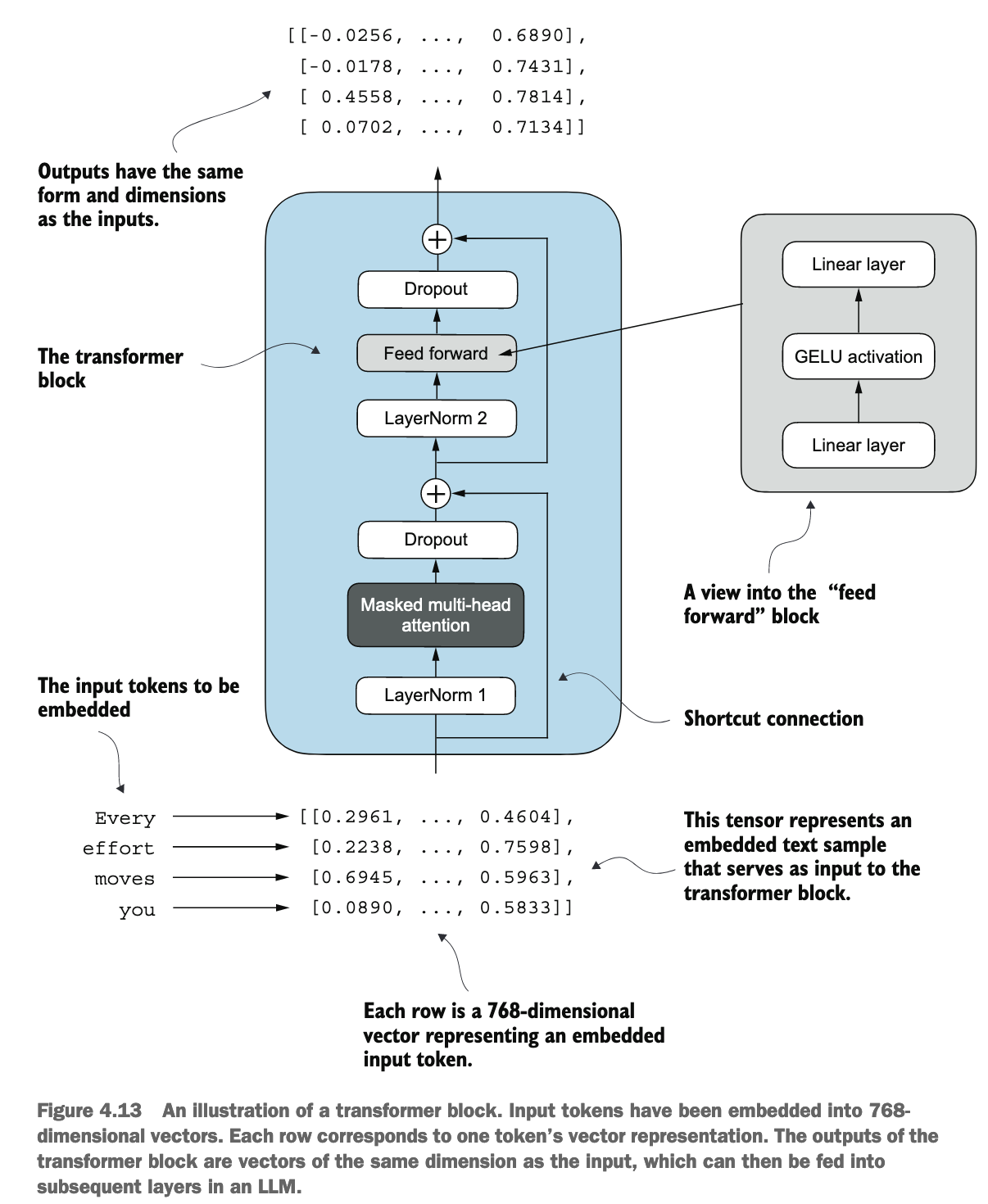
这张图展示了一个典型的Transformer解码器模块 (Transformer decoder block) 的结构，因为它包含了 “Masked Multi-head attention”。如果是编码器模块，通常会使用非掩码的多头注意力。不过，核心组件和流程是相似的。

整体流程概览：

输入是一系列词元（tokens）的嵌入向量（embedded vectors），每个词元都表示为一个768维的向量。这个Transformer模块会对这些输入向量进行一系列处理，最终输出同样形状和维度的向量，这些输出向量可以作为下一个Transformer模块的输入，或者用于最终的预测任务。

让我们按数据流动的顺序来分解：

1. Input Tokens (输入词元嵌入):

   • 图的左下角显示了 “Every effort moves you” 这句话被转换成了嵌入向量。
   • 作用：这是Transformer模块的起始输入。在自然语言处理中，原始文本（如单词或子词）首先会被转换成固定维度的向量表示，这些向量能够捕捉词元的语义信息。图中每个词元被表示为一个768维的向量。

2. Transformer Block (Transformer 模块) - 淡蓝色区域：

   这是核心处理单元，包含两个主要的子层（sub-layers）。

   第一个子层：Masked Multi-Head Attention (带掩码的多头注意力) 和相关组件

   • LayerNorm 1 (层归一化 1):
     • 作用：在将数据送入多头注意力机制之前，对其进行层归一化。层归一化是对每个样本（在这里是每个词元向量）的特征维度（768维）独立地进行归一化，使其均值为0，方差为1。
     • 目的：帮助稳定训练过程，加速收敛，并使得模型对权重的初始值不那么敏感。
   • Masked Multi-Head Attention (带掩码的多头注意力):
     • 作用：这是Transformer的核心组件之一，负责处理序列中不同词元之间的关系，并为每个词元生成一个考虑了上下文的新表示。
       • Multi-Head (多头)：它不是只计算一次注意力，而是将Query, Key, Value向量分割成多个“头”（heads），每个头并行地学习不同方面的注意力信息（即不同的表示子空间）。这使得模型能够同时关注来自不同位置、不同类型的相关信息。
       • Masked (掩码)：这里的“掩码”通常指因果掩码 (causal mask)。在生成任务（如语言模型预测下一个词）或解码器中，一个词元在计算其注意力时不应该“看到”它之后的词元。掩码操作会阻止当前位置关注未来位置的信息，确保了模型的自回归（auto-regressive）特性。
     • 目的：让模型理解句子中哪些词元对当前词元的含义最重要，并据此更新当前词元的表示。掩码确保了预测的有效性。
   • Dropout (紧随注意力层之后):
     • 作用：一种正则化技术。在训练过程中，它会以一定的概率随机地将一部分神经元的输出置为0。
     • 目的：防止模型过拟合，增强模型的泛化能力，通过阻止神经元之间形成过于复杂的共适应关系。
   • "+" (Shortcut Connection / Residual Connection - 快捷连接/残差连接):
     • 作用：将LayerNorm 1之前的输入（即第一个子层的原始输入，来自更早的嵌入或上一个模块的输出）与经过Dropout处理后的多头注意力层输出进行逐元素相加。
     • 目的：
       1. 缓解梯度消失：使得梯度能够更容易地流过深层网络。
       2. 简化学习：允许网络层（如注意力层）学习对输入的“残差”或修改，而不是学习一个全新的复杂映射。如果一个层没有学到有用的东西，它可以让残差趋近于0，信息就通过快捷连接原样传递。
       3. 训练更深的网络：这是ResNet等深层网络能够成功训练的关键技术。

   第二个子层：Feed Forward Network (前馈网络) 和相关组件

   • LayerNorm 2 (层归一化 2):

     • 作用：在将数据送入前馈网络之前，对第一个子层（注意力层+残差连接）的输出进行层归一化。
     • 目的：与LayerNorm 1类似，稳定数据分布，为后续的前馈网络提供良好状态的输入。

   • Feed Forward (前馈网络):

     • 图的右上角展示了其内部结构：“Linear layer -> GELU activation -> Linear layer”。
     • 作用：这是一个简单的全连接前馈神经网络，它独立地应用于序列中的每一个词元位置。
       • 第一个线性层 (Linear layer)：通常会将输入的维度（如768）扩展到一个更大的中间维度（如 768×4=3072）。
       • GELU activation (GELU激活函数)：引入非线性，GELU (Gaussian Error Linear Unit) 是一种常用的平滑激活函数。
       • 第二个线性层 (Linear layer)：再将维度从中间维度映射回原始维度（如 3072→768）。
     • 目的：在每个词元位置上进行更复杂的非线性变换，进一步处理和丰富词元的表示。它为模型提供了额外的计算能力和表示能力。注意力层负责混合序列中不同位置的信息，而前馈网络则在每个位置上独立地深化表示。

   • Dropout (紧随前馈网络之后):

     • 作用：与前面的Dropout层类似，对前馈网络的输出进行正则化。
     • 目的：防止过拟合。

   • "+" (Shortcut Connection / Residual Connection - 快捷连接/残差连接):

     • 作用：将LayerNorm 2之前的输入（即第二个子层的原始输入，来自第一个子层的输出）与经过Dropout处理后的前馈网络输出进行逐元素相加。
     • 目的：与第一个快捷连接类似，帮助训练，允许前馈网络学习对输入的残差修改。

3. Output (模块输出):

   • 图的顶部显示了输出的张量形式：“Outputs have the same form and dimensions as the inputs.”
   • 作用：经过Transformer模块的这两个子层处理后，每个输入词元的表示都得到了更新和丰富，同时保持了与输入相同的维度（768维）。这些输出向量可以被送入下一个Transformer模块进行进一步处理，或者在最后一个模块之后用于特定的下游任务（如分类、生成等）。

总结一下每个组件的核心价值：

• Embedding: 将离散的文本符号转化为连续的向量表示。
• Layer Normalization: 稳定每层（对每个样本而言）的输入，加速训练。
• Multi-Head Attention: 捕捉序列中词元间的长距离依赖和上下文关系，允许从多个角度理解信息。
• Masking (in Attention): 在解码器或自回归模型中，保证预测当前词时不依赖未来词。
• Feed Forward Network: 对每个词元的表示进行独立的非线性变换，增加模型容量。
• Shortcut/Residual Connections: 使得非常深的网络能够有效训练，缓解梯度消失，简化学习。
• Dropout: 防止模型过拟合，提高泛化能力。

Chapter 5

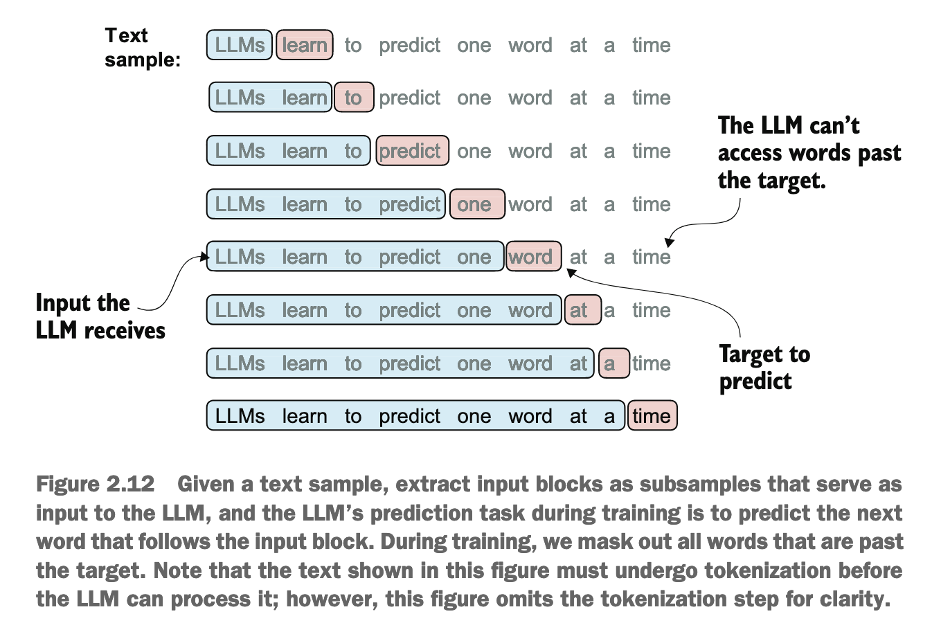
• 当模型的输入是 “every” 时（在序列 “every effort moves you” 的第一个位置），它应该预测的**目标（Target）**是 “effort”。所以模型会调整参数，使得在 “every” 位置输出的向量中，与 “effort” 对应的那个元素的值最大化。
• 当模型的输入是 “every effort” 时（模型在处理序列中 “effort” 这个位置时，通过因果掩码能看到 “every” 和 “effort”），它应该预测的目标是 “moves”。模型会调整参数，使得在 “effort” 位置输出的向量中，与 “moves” 对应的那个元素的值最大化。
• 当模型的输入是 “every effort moves” 时（模型在处理序列中 “moves” 这个位置时，能看到前三个词），它应该预测的目标是 “you”。模型会调整参数，使得在 “moves” 位置输出的向量中，与 “you” 对应的那个元素的值最大化。

总结与区分：

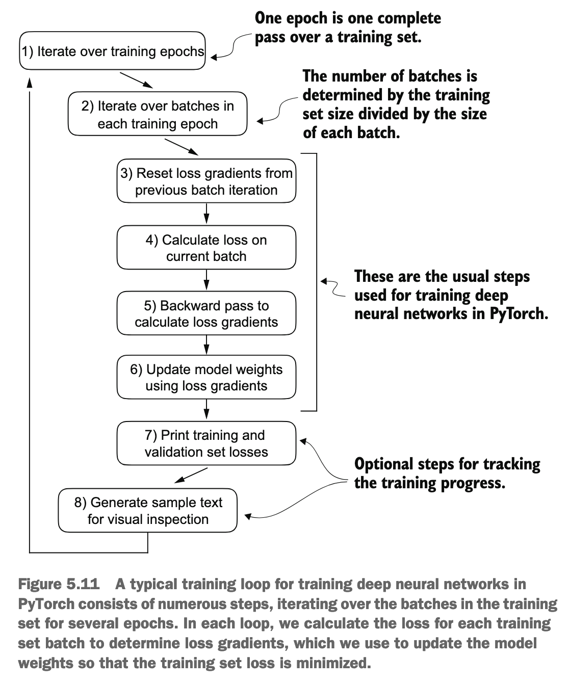
• 训练 (Training)：
  • 模型接收一段连续的文本序列作为输入（例如 “every effort moves you …")。
  • 对于输入序列中的每一个词元位置，模型都试图预测该位置之后紧跟着的那个真实的词元。
  • 这是通过并行计算完成的（得益于Transformer的架构），但因果掩码确保了预测的“公平性”（即预测位置 i 的词时，只使用 0…i 的信息）。
  • 因此，图示的不是一次输入三个词就并行预测三个独立的未来词，而是对于一个输入序列中的不同前缀（或不同位置），模型都在学习预测紧随其后的那个词。 图中的"Inputs"可以理解为不同时间点或不同上下文长度的输入状态，而"Targets"是对应这些状态的正确下一个词。
• 生成/推理 (Generation/Inference)：
  • 模型从一个初始词（或提示）开始。
  • 一次只预测一个下一个最可能的词。
  • 将这个预测出的词添加到输入序列中。
  • 以新的、更长的序列作为输入，再次预测下一个词。
  • 重复这个过程，直到生成结束标记或达到所需长度。

所以，图示更准确地反映了训练数据是如何组织和用于优化模型参数的：对于一个输入序列中的每个词，都有一个对应的“下一个词”作为标签。模型的目标是学习在给定前面的词（上下文）时，准确预测这个标签词。这种方式使得模型可以从大量文本中高效学习序列依赖关系。

Decoding strategies to control randomness

如果在生成 logits 后, 只使用 argmax, 那么每次都只会选择概率最大的, 这样随机性为 0, 我们可以将 argmax 换为 torch.multinomial, 采用概率性采样

• argmax 是一种确定性的选择方法：它总是选择概率最高的那个词元。这会导致生成的文本比较单调，缺乏变化，因为在相同的上下文中，它总是选择同一个词。
• torch.multinomial 是一种概率性的选择方法：它根据每个词元的概率大小进行采样。概率高的词更容易被选中，但概率低的词也有机会被选中。
  • 这使得生成的文本更加多样化和富有创造性，因为即使在相同的上下文中，模型也可能选择不同的下一个词

We can further control the distribution and selection process via a concept called temperature scaling. Temperature scaling is just a fancy description for dividing the logits by a number greater than 0:

def softmax_with_temperature(logits, temperature): 
 scaled_logits = logits / temperature
 return torch.softmax(scaled_logits, dim=0)

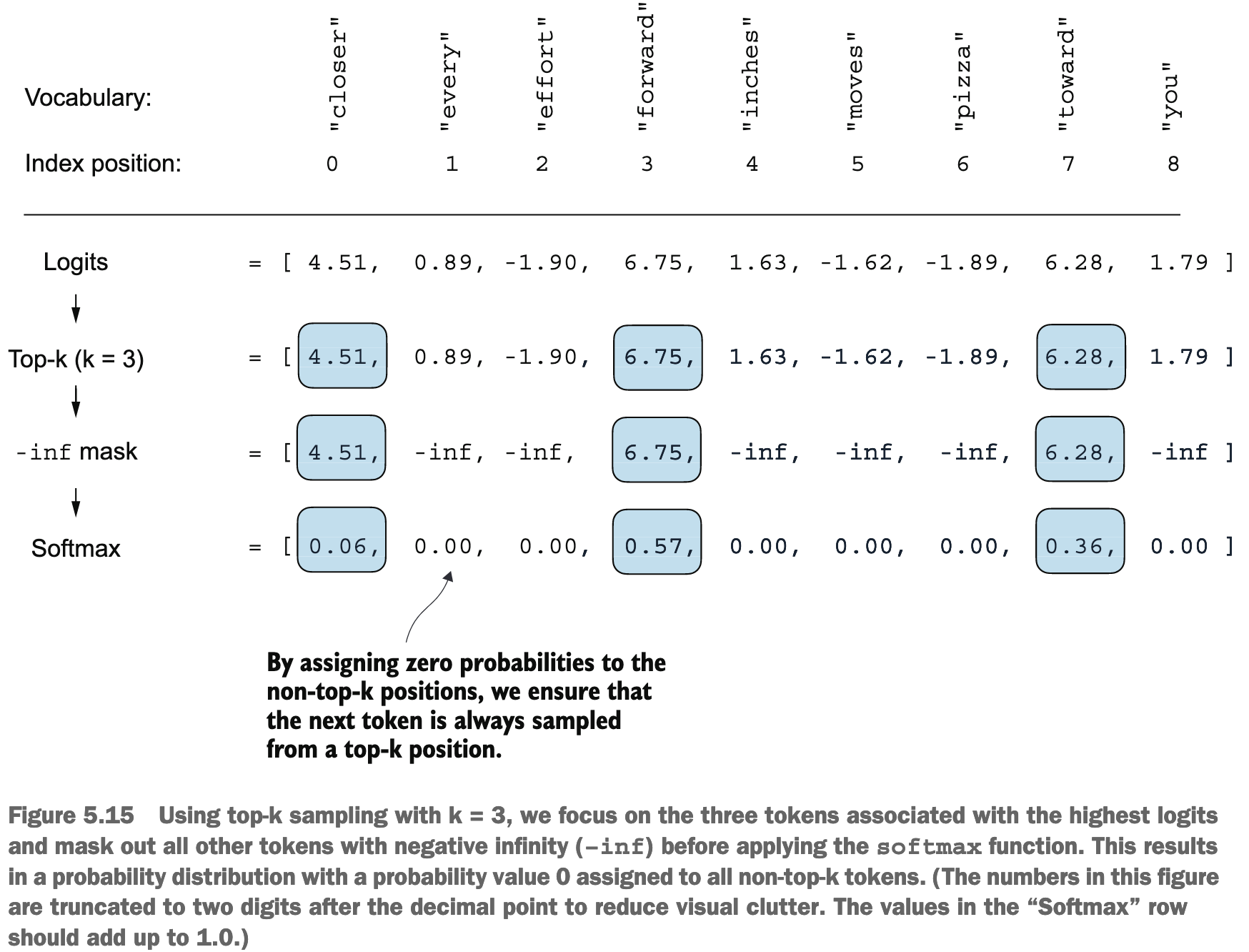
new_logits = torch.where( 
 condition=next_token_logits < top_logits[-1],
 input=torch.tensor(float('-inf')),
 other=next_token_logits 
)  
print(new_logits)

Chapter 6

在机器学习中，将数据集划分为训练集（Training Set）、验证集（Validation Set）和测试集（Testing Set）是一种标准的做法，目的是为了构建和评估一个稳健且泛化能力强的模型。这三个集合各自扮演着不同的关键角色：

1. 训练集 (Training Set - 70%)

   • 用途：训练模型。
   • 解释：这是数据集中最大的一部分，包含了模型将要学习的样本。模型会分析训练集中的数据，识别其中的模式、特征和关系。例如，在垃圾邮件分类任务中，模型会从训练集的邮件中学习哪些词语或特征通常与垃圾邮件相关联，哪些与正常邮件相关联。模型通过调整其内部参数（权重和偏差）来最小化在训练数据上的预测错误。

2. 验证集 (Validation Set - 10%)

   • 用途：调整模型超参数和进行模型选择。
   • 解释：在模型使用训练集训练了一轮或多轮之后，验证集被用来评估模型的表现。与训练集不同，模型在训练过程中并不能直接“看到”验证集的数据。验证集的主要作用有：
     • 超参数调优：机器学习模型有很多“超参数”（Hyperparameters），这些参数不是模型通过训练数据学到的，而是需要我们手动设置的（例如，学习率、树的深度、正则化强度等）。我们会尝试不同的超参数组合，用训练集训练模型，然后在验证集上评估哪组超参数能带来最好的性能。
     • 模型选择：如果你尝试了多种不同的模型架构（例如，决策树、支持向量机、神经网络），验证集可以帮助你比较这些模型在未见过数据上的表现，从而选择最优的模型。
     • 防止过拟合：模型在训练集上表现很好，但在新数据上表现差的现象称为过拟合 (Overfitting)。验证集可以帮助我们监控模型是否开始过拟合。如果在训练集上性能持续提升，但在验证集上性能开始下降，就可能意味着模型过拟合了，需要采取措施（如提前停止训练、增加正则化等）。

3. 测试集 (Testing Set - 20%)

   • 用途：对最终选定的模型进行无偏评估。
   • 解释：测试集是“神圣不可侵犯”的，它在整个模型训练和调优过程中都不能被模型“看到”或用来做任何决策。只有当你完成了所有的模型训练、超参数调整和模型选择后，才会使用测试集来评估最终模型的性能。
     • 无偏评估：因为模型从未接触过测试集的数据，所以测试集上的性能可以被认为是模型在真实世界中对全新、未知数据表现的一个公正的、无偏的估计。
     • 最终性能指标：测试集上的准确率、精确率、召回率、F1分数等指标，通常被用作衡量模型最终好坏的关键指标。

总结一下它们的作用流程：

1. 用训练集喂给模型，让模型学习。
2. 用验证集调整模型的各种设置（超参数），选择最好的模型配置，并监控是否过拟合。
3. 一旦模型训练和调整完毕，就用测试集进行一次最终的、独立的评估，看看模型在真实应用场景中可能会表现如何。

Chapter 7

Fine-tune instructions 的特殊之处在于:

1. 对于同一个 batch, 我们需要 padding 到同一个长度 (使用 endoftext)
2. target 也是 shift 一个 token
3. 我们只保留一个 endoftext 标志, 后续的 endoftext 需要被替换为 -100 (pytorch 的 cross_entry 计算时会忽略这个 id)

所以在定义 Dataset 时, 只定义了 encoded_texts, 没有生成 target 之类的,需要在 loader 时统一处理:

class InstructionDataset(Dataset):
    def __init__(self, data, tokenizer):
        self.data = data

        # Pre-tokenize texts
        self.encoded_texts = []
        for entry in data:
            instruction_plus_input = format_input(entry)
            response_text = f"\n\n### Response:\n{entry['output']}"
            full_text = instruction_plus_input + response_text
            self.encoded_texts.append(
                tokenizer.encode(full_text)
            )

    def __getitem__(self, index):
        return self.encoded_texts[index]

    def __len__(self):
        return len(self.data)

按照 batch 来 padding:

def custom_collate_fn(
    batch,
    pad_token_id=50256,
    ignore_index=-100,
    allowed_max_length=None,
    device="cpu"
):
    # Find the longest sequence in the batch
    batch_max_length = max(len(item)+1 for item in batch)

    # Pad and prepare inputs and targets
    inputs_lst, targets_lst = [], []

    for item in batch:
        new_item = item.copy()
        # Add an <|endoftext|> token
        new_item += [pad_token_id]
        # Pad sequences to max_length
        padded = (
            new_item + [pad_token_id] *
            (batch_max_length - len(new_item))
        )
        inputs = torch.tensor(padded[:-1])  # Truncate the last token for inputs
        targets = torch.tensor(padded[1:])  # Shift +1 to the right for targets

        # New: Replace all but the first padding tokens in targets by ignore_index
        # 这个表达式会创建一个新的 PyTorch 张量，其形状与 targets 相同
        # 新张量中的每个元素都是一个布尔值 (True 或 False)
        # 表示 targets 中对应位置的元素是否等于 pad_token_id
        mask = targets == pad_token_id
        # 它接收一个布尔张量 (mask) 作为输入，并返回一个包含所有 True 元素的索引的张量
        indices = torch.nonzero(mask).squeeze()
        if indices.numel() > 1:
            # indices 存的是所有 padding token 的位置
            # targets[indices] 就可以直接批量修改
            targets[indices[1:]] = ignore_index

        # New: Optionally truncate to maximum sequence length
        if allowed_max_length is not None:
            inputs = inputs[:allowed_max_length]
            targets = targets[:allowed_max_length]

        inputs_lst.append(inputs)
        targets_lst.append(targets)

    # Convert list of inputs and targets to tensors and transfer to target device
    inputs_tensor = torch.stack(inputs_lst).to(device)
    targets_tensor = torch.stack(targets_lst).to(device)

    return inputs_tensor, targets_tensor

• Another additional detail of the previous custom_collate_fn function is that we now directly move the data to the target device (e.g., GPU) instead of doing it in the main training loop, which improves efficiency because it can be carried out as a background process when we use the custom_collate_fn as part of the data loader