1-builtin-tutorial

Background

GPU Memory Model

SRAM (Static RAM)
- Located inside the GPU core, it utilizes Registers, L1 Cache, and L2 Cache:
- Registers — These are tiny, ultra-fast memory locations within each GPU core. Registers store immediate values that a core is actively processing, making them the fastest type of memory.
- L1 Cache — This is the first-level cache inside a Streaming Multiprocessor (SM). It stores frequently accessed data to speed up calculations and reduce access to slower memory (like DRAM).
- L2 Cache — This is a larger, second-level cache that is shared across multiple SMs. It helps store and reuse data that might not fit in L1 cache, reducing reliance on external memory (VRAM).
HBM
- Bigger capacity

pasted-image-20260107162911

pasted-image-20260107162847

GPU Architecture

GPU
 └── SM × N (e.g., 108 on A100)
      └── Warp Schedulers × 4 (每个SM)
           └── Warp × 多个 (每个SM可同时驻留多个warps)
                └── Threads × 32 (固定，一个warp)

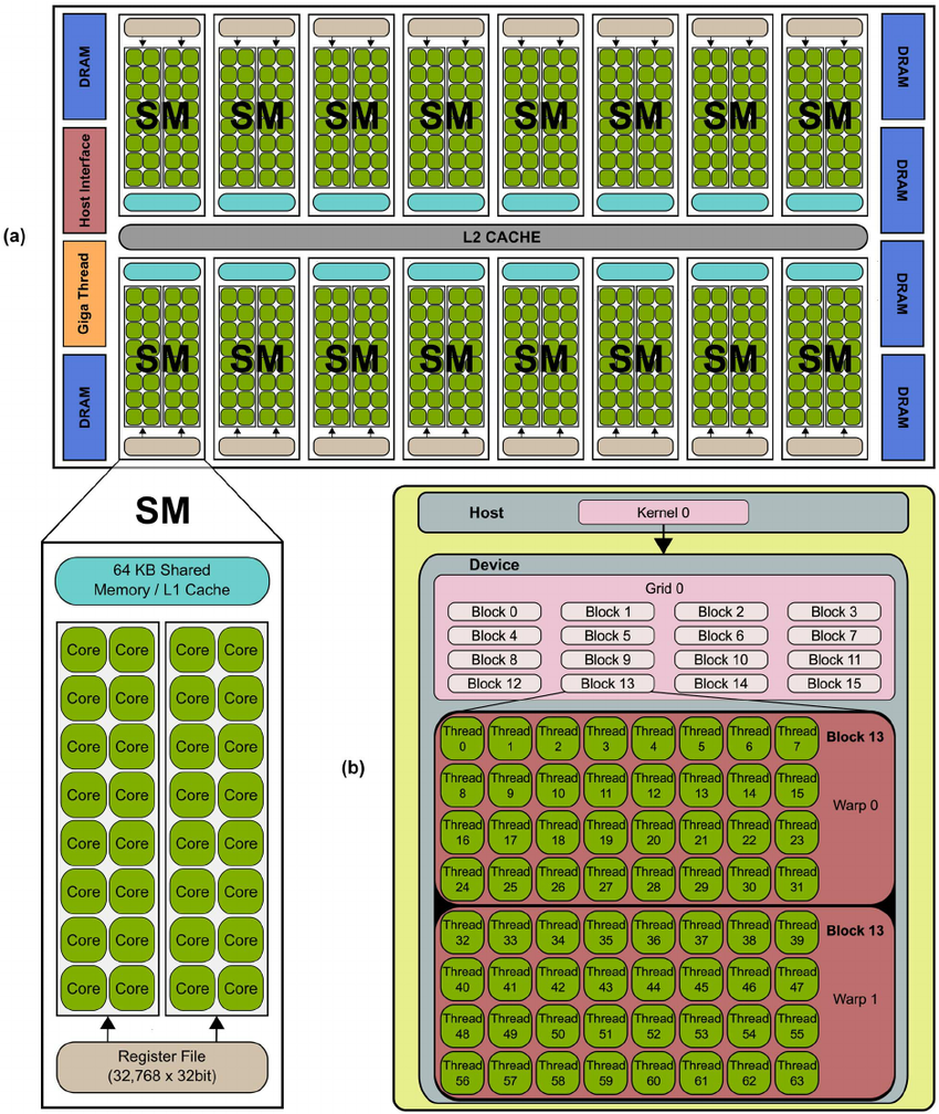
Streaming Multiprocessor

A Streaming Multiprocessor (SM) is the fundamental processing unit of a GPU.

pasted-image-20260107163232

Each SM contains multiple GPU cores, a small memory pool (SRAM), and execution units.
Each SM operates independently, handling multiple programs in parallel.
The number of SMs in a GPU directly affects its computational power.

When a program runs on a GPU, it gets split across multiple SMs, and each SM works on a chunk of data. More SMs mean better performance.

Cores and Warps

GPU Cores: The Smallest Compute Unit

A core is the smallest unit of computation in a GPU.
Unlike CPU cores, GPU cores are optimized for Floating Point Operations (FLOPs).
Each core can perform one FLOP per cycle.

Warps: Groups of GPU Cores

GPU cores are grouped into warps.
Nvidia GPUs have 32 cores per warp, while AMD GPUs have 64 cores per warp.
All cores in a warp must execute the same instruction simultaneously but operate on different data.

CUDA Model

一个 Block 被调度到一个 SM 上执行
同一 Block 内的所有 threads 共享该 SM 的 Shared Memory
不同 Blocks 之间无法直接通信（除非通过 global memory）

Example:

Grid (整个 kernel 启动)
  └─ Blocks (多个独立的工作组)
       └─ Threads (Block 内的并行线程)

__global__ void vectorAdd(const float *A, const float *B, float *C, int n) {
    // 计算当前线程对应的全局索引
    int idx = blockIdx.x * blockDim.x + threadIdx.x;
    
    // 边界检查:确保不越界
    if (idx < n) {
        C[idx] = A[idx] + B[idx];
    }
}

int threadsPerBlock = 256;
int blocksPerGrid = (n + threadsPerBlock - 1) / threadsPerBlock;
vectorAdd<<<blocksPerGrid, threadsPerBlock>>>(d_A, d_B, d_C, n);

在写 CUDA 代码时，需要以 Threads 作为视角

Triton Model

CUDA:     Grid → Blocks → Warps (32 threads) → Threads
                  ↓
Triton:   Grid → Programs → [自动 vectorization]

Triton 隐藏了 Warp 和 Thread 的细节，让你只需关注 Program 级别的并行。

每个 Program 是一个独立的执行单元：

处理一块连续的数据（如 1024 个元素）
在一个 SM 上执行
Program 之间完全独立，无法通信

概念	CUDA	Triton
Grid Dimensions	`gridDim`	`grid=` 参数
Block Index	`blockIdx`	`tl.program_id()`
Block Dimensions	`blockDim` (threads per block)	隐藏 (由编译器根据 `BLOCK_SIZE` 决定)
Thread Index	`threadIdx`	隐藏
Shared Memory	手动管理 (`__shared__`)	隐藏 (编译器自动管理)

1-Vector Addition

向量级别的操作非常符合直觉，把一个向量按照 BLOCK_SIZE 进行切分，同时执行多个 program, 每个 program 只负责 BLOCK_SIZE 个数据

import torch

import triton
import triton.language as tl

DEVICE = triton.runtime.driver.active.get_active_torch_device()


@triton.jit
def add_kernel(x_ptr,  # *Pointer* to first input vector.
               y_ptr,  # *Pointer* to second input vector.
               output_ptr,  # *Pointer* to output vector.
               n_elements,  # Size of the vector.
               BLOCK_SIZE: tl.constexpr,  # Number of elements each program should process.
               # NOTE: `constexpr` so it can be used as a shape value.
               ):
    # There are multiple 'programs' processing different data. We identify which program
    # we are here:
    pid = tl.program_id(axis=0)  # We use a 1D launch grid so axis is 0.
    # This program will process inputs that are offset from the initial data.
    # For instance, if you had a vector of length 256 and block_size of 64, the programs
    # would each access the elements [0:64, 64:128, 128:192, 192:256].
    # Note that offsets is a list of pointers:
    block_start = pid * BLOCK_SIZE
    offsets = block_start + tl.arange(0, BLOCK_SIZE)
    # Create a mask to guard memory operations against out-of-bounds accesses.
    mask = offsets < n_elements
    # Load x and y from DRAM, masking out any extra elements in case the input is not a
    # multiple of the block size.
    x = tl.load(x_ptr + offsets, mask=mask)
    y = tl.load(y_ptr + offsets, mask=mask)
    output = x + y
    # Write x + y back to DRAM.
    tl.store(output_ptr + offsets, output, mask=mask)

2-Fused Softmax

二维矩阵就会涉及到如何切分了，或者说每个 Program 负责哪个部分

Vector Addition:

1D 问题：直接映射到一维数组
每个元素独立：c[i] = a[i] + b[i]
数据量：假设 100,000 个元素
策略：启动 100 个 programs，每个处理 1000 个元素

Softmax:

2D 问题：按行计算（每行内的元素有依赖关系）
每行需要：max → exp → sum → divide
数据量：假设 10,000 行，每行 1024 个元素
问题：是否启动 10,000 个 programs？

启动 10000 个 Programs 的开销太大了

这里其实涉及到两个范式：

Fixed-Size Grid
Grid-Stride Loop

@triton.jit
def fixed_grid_kernel(data_ptr, n_elements, BLOCK_SIZE: tl.constexpr):
    # 获取当前 program ID
    pid = tl.program_id(0)
    
    # 计算当前 program 负责的元素范围
    offsets = pid * BLOCK_SIZE + tl.arange(0, BLOCK_SIZE)
    mask = offsets < n_elements
    
    # 加载数据
    data = tl.load(data_ptr + offsets, mask=mask)
    
    # 处理数据
    result = process(data)
    
    # 存储结果
    tl.store(data_ptr + offsets, result, mask=mask)

# 调用：grid size 根据数据量计算
n_elements = 10000
BLOCK_SIZE = 1024
grid = (triton.cdiv(n_elements, BLOCK_SIZE),)  # = 10 个 programs
fixed_grid_kernel[grid](data, n_elements, BLOCK_SIZE)

@triton.jit
def grid_stride_kernel(data_ptr, n_elements, BLOCK_SIZE: tl.constexpr):
    # 获取当前 program ID 和总 program 数
    pid = tl.program_id(0)
    num_programs = tl.num_programs(0)
    
    # 计算需要处理的总 block 数
    n_blocks = triton.cdiv(n_elements, BLOCK_SIZE)
    
    # 循环处理分配给当前 program 的所有 blocks
    for block_idx in range(pid, n_blocks, num_programs):
        # 计算当前 block 的元素范围
        offsets = block_idx * BLOCK_SIZE + tl.arange(0, BLOCK_SIZE)
        mask = offsets < n_elements
        
        # 加载数据
        data = tl.load(data_ptr + offsets, mask=mask)
        
        # 处理数据
        result = process(data)
        
        # 存储结果
        tl.store(data_ptr + offsets, result, mask=mask)

# 调用：grid size 固定
n_elements = 10000
BLOCK_SIZE = 1024
grid = (256,)  # 固定 256 个 programs
grid_stride_kernel[grid](data, n_elements, BLOCK_SIZE)

对于 Fixed-Size Grid 来说，每个 Program 只处理一个 Block; 但是对于 Grid-Stride Loop 来说，每个 Program 需要处理多个 Block

# Fixed-Size Grid

grid = (10,)  # 启动 10 个 programs

Program 0 → Block 0 (元素 0-1023)
Program 1 → Block 1 (元素 1024-2047)
Program 2 → Block 2 (元素 2048-3071)
...
Program 9 → Block 9 (元素 9216-9999)

每个 program 处理 1 个 block 后结束

# Grid-Stride Loop

grid = (4,)  # 只启动 4 个 programs

Program 0 → Block 0, Block 4, Block 8  (循环 3 次)
Program 1 → Block 1, Block 5, Block 9  (循环 3 次)
Program 2 → Block 2, Block 6           (循环 2 次)
Program 3 → Block 3, Block 7           (循环 2 次)

每个 program 通过循环处理多个 blocks

考虑 Grid-Stride Loop 中的下面这个循环：

# 没有 pipelining 的执行
for i in range(10):
    data = load_from_memory(i)     # 等待 ~200 cycles
    result = compute(data)          # 计算 ~10 cycles
    store_to_memory(result, i)      # 等待 ~200 cycles
    
# 大部分时间在等待内存！

我们可以同时处理 3 个迭代的不同阶段

迭代 0: [加载 0]
迭代 1: [加载 1] [计算 0]
迭代 2: [加载 2] [计算 1] [存储 0]
迭代 3:          [计算 2] [存储 1] ← 加载迭代 3
迭代 4:                   [存储 2] ← 计算迭代 3 ← 加载迭代 4

在 Triton 中可以使用 Software Pipeline:

@triton.jit
def kernel_with_pipelining(data_ptr, n_elements, BLOCK_SIZE: tl.constexpr, num_stages: tl.constexpr):
    pid = tl.program_id(0)
    num_programs = tl.num_programs(0)
    n_blocks = triton.cdiv(n_elements, BLOCK_SIZE)
    
    # 关键：在 tl.range 中指定 num_stages
    for block_idx in tl.range(pid, n_blocks, num_programs, num_stages=num_stages):
        offsets = block_idx * BLOCK_SIZE + tl.arange(0, BLOCK_SIZE)
        mask = offsets < n_elements
        
        # 这些操作会被自动流水线化
        data = tl.load(data_ptr + offsets, mask=mask)  # Stage 1: Load
        result = process(data)                          # Stage 2: Compute
        tl.store(data_ptr + offsets, result, mask=mask) # Stage 3: Store

# 使用
grid = (256,)
kernel_with_pipelining[grid](data, n_elements, BLOCK_SIZE=1024, num_stages=3)

知道这些背景知识后，我们再来看 Fused Softmax 的实现：

@triton.jit
def softmax_kernel(output_ptr, input_ptr, input_row_stride, output_row_stride, n_rows, n_cols, BLOCK_SIZE: tl.constexpr, num_stages: tl.constexpr):
    # starting row of the program
    row_start = tl.program_id(0)
    row_step = tl.num_programs(0)
    for row_idx in tl.range(row_start, n_rows, row_step, num_stages=num_stages):
        # The stride represents how much we need to increase the pointer to advance 1 row
        row_start_ptr = input_ptr + row_idx * input_row_stride
        # The block size is the next power of two greater than n_cols, so we can fit each
        # row in a single block
        col_offsets = tl.arange(0, BLOCK_SIZE)
        input_ptrs = row_start_ptr + col_offsets
        # Load the row into SRAM, using a mask since BLOCK_SIZE may be > than n_cols
        mask = col_offsets < n_cols
        row = tl.load(input_ptrs, mask=mask, other=-float('inf'))
        # Subtract maximum for numerical stability
        row_minus_max = row - tl.max(row, axis=0)
        # Note that exponentiation in Triton is fast but approximate (i.e., think __expf in CUDA)
        numerator = tl.exp(row_minus_max)
        denominator = tl.sum(numerator, axis=0)
        softmax_output = numerator / denominator
        # Write back output to DRAM
        output_row_start_ptr = output_ptr + row_idx * output_row_stride
        output_ptrs = output_row_start_ptr + col_offsets
        tl.store(output_ptrs, softmax_output, mask=mask)

对于教程中 Wrapper 的思路，这里就先不分析了

3-Matrix Multiplication

Roughly speaking, the kernel that we will write will implement the following blocked algorithm to multiply a (M, K) by a (K, N) matrix:

# Do in parallel
for m in range(0, M, BLOCK_SIZE_M):
  # Do in parallel
  for n in range(0, N, BLOCK_SIZE_N):
    acc = zeros((BLOCK_SIZE_M, BLOCK_SIZE_N), dtype=float32)
    for k in range(0, K, BLOCK_SIZE_K):
      a = A[m : m+BLOCK_SIZE_M, k : k+BLOCK_SIZE_K]
      b = B[k : k+BLOCK_SIZE_K, n : n+BLOCK_SIZE_N]
      acc += dot(a, b)
    C[m : m+BLOCK_SIZE_M, n : n+BLOCK_SIZE_N] = acc

X[i, j] is given by &X[i, j] = X + i*stride_xi + j*stride_xj

&A[m : m+BLOCK_SIZE_M, k:k+BLOCK_SIZE_K] =  
 a_ptr + (m : m+BLOCK_SIZE_M)[:, None]*A.stride(0) + (k : k+BLOCK_SIZE_K)[None, :]*A.stride(1);
&B[k : k+BLOCK_SIZE_K, n:n+BLOCK_SIZE_N] =  
 b_ptr + (k : k+BLOCK_SIZE_K)[:, None]*B.stride(0) + (n : n+BLOCK_SIZE_N)[None, :]*B.stride(1);

从 A @ B = C 视角出发

C[i,j] = A[i,:] * B[:,j]

# 一种最简单的排布方式就是：
pid = tl.program_id(axis=0)
grid_n = tl.cdiv(N, BLOCK_SIZE_N)
pid_m = pid // grid_n
pid_n = pid % grid_n 

# 比如 pid = 7，矩阵为 (4, 3)
# 7 就应该对应 (7//3 = 2, 7%3=1) => (2,1)

如果这么遍历 C[0,0] -> C[0, N] -> C[M,0] -> C[M, N] 的话，L2 Cache 没有得到充分利用，还存在一种更好的方式：

pasted-image-20260108212532

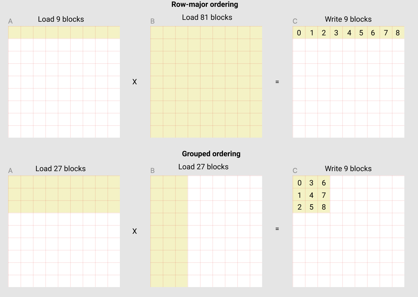
还可以换个方式理解，如果在 Row-major ordering 的情况下要复用，那我们需要整个 B 矩阵保存在 SRAM 中才行，比如 A 的第二行就可以复用整个 B 矩阵
但是用 Grouped ordering，算这 9 块时内部就能复用

Important

Row-major ordering 就是通常意义上的 row-major ordering
图中的 Grouped ordering 其实是 Grouped + colunm-major ordering
- 所以在计算下标时，需要涉及到先分组（横向切分）再 colunm-major 排序

相当于是要想一个算法，把

1 => (1, 0)
4 => (1, 1)
5 => (2, 1)
6 => (0, 3)

上去

由于在 C 中，横向的数字是连续，所以我们可以划分为一个 GROUP，所以一个 GROUP 大小为 GROUP_SIZE_M * num_pid_n

pid=0  pid=4  pid=8  pid=12 pid=16 pid=20 pid=24 pid=28
  ↓      ↓      ↓      ↓      ↓      ↓      ↓      ↓
┌────┬────┬────┬────┬────┬────┬────┬────┐
│ 0  │ 4  │ 8  │12  │16  │20  │24  │28  │ ← 行0
├────┼────┼────┼────┼────┼────┼────┼────┤
│ 1  │ 5  │ 9  │13  │17  │21  │25  │29  │ ← 行1
├────┼────┼────┼────┼────┼────┼────┼────┤
│ 2  │ 6  │10  │14  │18  │22  │26  │30  │ ← 行2
├────┼────┼────┼────┼────┼────┼────┼────┤
│ 3  │ 7  │11  │15  │19  │23  │27  │31  │ ← 行3
└────┴────┴────┴────┴────┴────┴────┴────┘


C 矩阵（12 行 × 8 列 blocks）：

           8 列（num_pid_n = 8）
        ←―――――――――――――――→
      ┌────────────────────┐ ↑
      │    Group 0         │ │
      │  (32 个 programs)  │ │ 4行
      │                    │ │ (GROUP_SIZE_M)
      ├────────────────────┤ ↓
      │    Group 1         │ ↑
      │  (32 个 programs)  │ │ 4行
      │                    │ │
      ├────────────────────┤ ↓
      │    Group 2         │ ↑
      │  (32 个 programs)  │ │ 4行
      │                    │ │
      └────────────────────┘ ↓

在一个 (m, n) 的矩阵中，如果是 row-major:

pid_m = pid // num_pid_n
pid_n = pid % num_pid_n


num_pid_m = 2
num_pid_n = 4
0 1 2 3
4 5 6 7

pid = 6 
pid_m = 6 // 4 = 1
pid_n = 6 %  4 = 2

如果是 colunm-major:

pid_m = pid % num_pid_m
pid_n = pid // num_pid_m

num_pid_m = 2
num_pid_n = 4
0 2 4 6
1 3 5 7

pid = 5 
pid_m = 5 % 2 = 1
pid_n = 5 // 2 = 2

下面的代码中其实就采用了 colunm-major

注意 group_size_m 是为了处理最后一个 group 可能不完整的边界情况

假设：

num_pid_m = 10（C 矩阵有 10 行 blocks）
GROUP_SIZE_M = 4（每个 group 想包含 4 行）
最后一个 group 应该只有 2 行

# Program ID
pid = tl.program_id(axis=0)
# Number of program ids along the M axis
num_pid_m = tl.cdiv(M, BLOCK_SIZE_M)
# Number of programs ids along the N axis
num_pid_n = tl.cdiv(N, BLOCK_SIZE_N)
# Number of programs in group
num_pid_in_group = GROUP_SIZE_M * num_pid_n
# Id of the group this program is in
group_id = pid // num_pid_in_group
# Row-id of the first program in the group
first_pid_m = group_id * GROUP_SIZE_M
# If `num_pid_m` isn't divisible by `GROUP_SIZE_M`, the last group is smaller
group_size_m = min(num_pid_m - first_pid_m, GROUP_SIZE_M)
# *Within groups*, programs are ordered in a column-major order
# Row-id of the program in the *launch grid*
pid_m = first_pid_m + ((pid % num_pid_in_group) % group_size_m)
# Col-id of the program in the *launch grid*
pid_n = (pid % num_pid_in_group) // group_size_m

接下来是指针算术部分：

# `a_ptrs` is a block of [BLOCK_SIZE_M, BLOCK_SIZE_K] pointers
# `b_ptrs` is a block of [BLOCK_SIZE_K, BLOCK_SIZE_N] pointers
# See above `Pointer Arithmetic` section for details
offs_am = (pid_m * BLOCK_SIZE_M + tl.arange(0, BLOCK_SIZE_M)) % M
offs_bn = (pid_n * BLOCK_SIZE_N + tl.arange(0, BLOCK_SIZE_N)) % N
offs_k = tl.arange(0, BLOCK_SIZE_K)
a_ptrs = a_ptr + (offs_am[:, None] * stride_am + offs_k[None, :] * stride_ak)
b_ptrs = b_ptr + (offs_k[:, None] * stride_bk + offs_bn[None, :] * stride_bn)
"""
    [:, None] turns [m1,m2,m3] into [[m1],[m2],[m3]] 
    [None, :] turns [n1,n2,n3] into [[n1,n2,n3]]
    combining them gives the matrix
    [[m1n1, m1n2, m1n3],
     [m2n1, m2n2, m2n3],
     [m3n1, m3n2, m3n3]] 
"""

要加载一个二维矩阵，你也必须提供一个二维指针
这里可以认为是进行了一次广播

比如:

M = 9
N = 9

 0  1  2  3  4  5  6  7  8
 9 10 11 12 13 14 15 16 17
18 19 20 21 22 23 24 25 26
27 28 29 30 31 32 33 34 35
36 37 38 39 40 41 42 43 44
45 46 47 48 49 50 51 52 53
54 55 56 57 58 59 60 61 62
63 64 65 66 67 68 69 70 71
72 73 74 75 76 77 78 79 80

stride_am = 9
stride_ak = 1
stride_bk = 9
stride_bn = 1

offs_am = [0:3]
offs_k = [0:3]
offs_bn = [0:3]

offs_am[:, None] * stride_am -> [[0], [1], [2]] * stride_am -> [[0], [9], [18]]
offs_k[None, :] * stride_ak -> [[0, 1, 2]] * 1

[[0], [9], [18]] + [[0, 1, 2]] ->
array([[ 0,  1,  2],
       [ 9, 10, 11],
       [18, 19, 20]])

最后是核心计算部分：

 accumulator = tl.zeros((BLOCK_SIZE_M, BLOCK_SIZE_N), dtype=tl.float32)
for k in range(0, tl.cdiv(K, BLOCK_SIZE_K)):
 # Load the next block of A and B, generate a mask by checking the K dimension.
 # If it is out of bounds, set it to 0.
 a = tl.load(a_ptrs, mask=offs_k[None, :] < K - k * BLOCK_SIZE_K, other=0.0)
 b = tl.load(b_ptrs, mask=offs_k[:, None] < K - k * BLOCK_SIZE_K, other=0.0)
 # We accumulate along the K dimension.
 accumulator = tl.dot(a, b, accumulator)
 # Advance the ptrs to the next K block.
 a_ptrs += BLOCK_SIZE_K * stride_ak
 b_ptrs += BLOCK_SIZE_K * stride_bk
# You can fuse arbitrary activation functions here
# while the accumulator is still in FP32!
if ACTIVATION == "leaky_relu":
 accumulator = leaky_relu(accumulator)
c = accumulator.to(tl.float16)

# -----------------------------------------------------------
# Write back the block of the output matrix C with masks.
offs_cm = pid_m * BLOCK_SIZE_M + tl.arange(0, BLOCK_SIZE_M)
offs_cn = pid_n * BLOCK_SIZE_N + tl.arange(0, BLOCK_SIZE_N)
c_ptrs = c_ptr + stride_cm * offs_cm[:, None] + stride_cn * offs_cn[None, :]
c_mask = (offs_cm[:, None] < M) & (offs_cn[None, :] < N)
tl.store(c_ptrs, c, mask=c_mask)

$$\text{TPOT}(t) = k_1 \cdot \log(t) + b_1 \quad \text{(2个参数)}$$$$\text{TTFT}(s, t) = k_2 \cdot \log(t) + k_3 \cdot \log(s) + b_2 \quad \text{(3个参数)}$$

Background#

GPU Memory Model#

GPU Architecture#

Streaming Multiprocessor#

Cores and Warps#

CUDA Model#

Triton Model#

1-Vector Addition#

2-Fused Softmax#

3-Matrix Multiplication#

Background

GPU Memory Model

GPU Architecture

Streaming Multiprocessor

Cores and Warps

CUDA Model

Triton Model

1-Vector Addition

2-Fused Softmax

3-Matrix Multiplication