Extensive Reading
Author Info
- About me - Xunhao Lai
- Good at writing Triton, here is another repo: XunhaoLai/native-sparse-attention-triton: Efficient triton implementation of Native Sparse Attention.
Background
As LLM context windows expand (up to 1M+ tokens), the pre-filling phase (processing the input prompt) becomes prohibitively expensive due to the quadratic complexity of full attention($O(n^2)$).
Why prior sparse attention is insufficient
Many approaches use fixed sparse patterns (e.g., sliding window) or offline-discovered patterns/ratios. These often fail because:
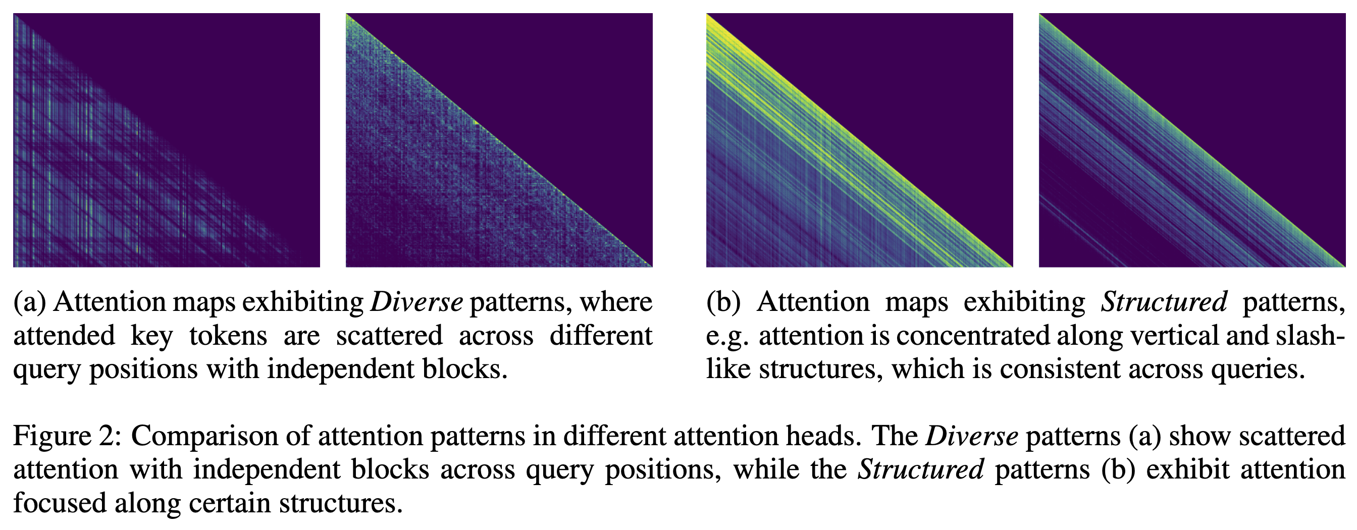
Attention patterns differ by head: some heads show scattered, query-dependent blocks (“Diverse”), while others follow stable structures (“Structured / Vertical-Slash”).
Sparsity needs differ by input: harder samples (long-range dependencies) need more computation than easier ones.
Insights
Classify attention heads into two types, and use an online sparse prefill mechanism that adapts:
- Which sparse pattern to use per attention head (and per input)
- How many query–key blocks to compute (dynamic budget) per head, per input
Approaches
FlexPrefill dynamically classifies each attention head (for the current input) into:
- Query-Aware head: attention varies across query positions; needs query-specific estimation
- Vertical-Slash head: attention follows a stable “vertical + slash” structure that can be inferred from a small sample and then expanded
Two components:
- Query-Aware Sparse Pattern Determination to determine which pattern to use per attention head
- Cumulative-Attention Based Index Selection to determine how many query-key blocks to compute
两个组件都是在真正的注意力计算之前进行估算,所以必须想办法降低这部分的计算开销,阅读时可以重点关注一下是通过哪些方法来估算的
Query-Aware Sparse Pattern Determination
取真实 Query 的最后一个 Block
先得到一个估算分布
$$\bar{a} = \text{softmax}(\text{avgpool}(\hat{Q}) \cdot \text{avgpool}(K)^\top / \sqrt{d})$$avgpool(Q)指的是对 Q 进行平均池化,把序列中每 BLOCK_SIZE 个连续的 token 合并为一个平均向量,减小矩阵的尺寸- 在这个缩小版的矩阵上做点积和 softmax
然后在计算一个真实分布
$$\hat{a} = \text{sumpool}(\text{softmax}(\hat{Q} \cdot K^\top / \sqrt{d}))$$sumpool():把算出来的分数按块(Block)进行求和。
最后计算这两个分布之间的 Jensen-Shannon 散度(差异度):
- 如果 $\bar{a}$ 和 $\hat{a}$ 差异小:说明“平均池化”这个偷懒的方法是有效的,我们可以放心地用低成本的 $\bar{a}$ 这种方法去处理所有的 Query,从而快速找到稀疏注意力的位置(即 Query-Aware 模式)。
- 如果 $\bar{a}$ 和 $\hat{a}$ 差异大:说明当前的注意力模式很精细或很特殊,光看“平均值”会看走眼(比如某个块平均值很低,但里面藏着一个极其重要的 token)。这时候估算不可靠,系统就放弃估算,转而使用固定的 Vertical-Slash 模式(保留最近的内容和特定的垂直线)。
- 这里可能要理解一下,第一次看的时候,直觉认为如果两个分布之间的差异不大,说明比较的结构化,应该更像 Vertical-Slash 模式
- 其实关键在于,:FlexPrefill 中的“Query-Aware”模式并不是指“最精细的模式”,而是指“依赖估算结果的模式”
- 可以想一下:什么情况下估算分布会失效 -> 某个特定的 Token 块非常重要,但是在池化之后重要性被抹掉了,所以这时就必须使用 Vertical-Slash 来选择出这些 Token
Cumulative-Attention Based Index Selection
判断每个头属于什么类型是第一步,第二步我们要根据 attn head 的类型确定具体的稀疏注意力计算方式,具体来说就是选择哪些 Q-K block 进行计算
论文给出的概览还是比较清晰的
- Query-Aware head
- 把原始的 Q,K 做池化,然后计算得到一个粗粒度的注意力矩阵
- 把这个二维的注意力矩阵 flatten, 并再次归一化,使得所有元素之和为 1
- 从大到小进行排序,进行累加,直到累加分数超过 $\gamma$
- 输出最后的稀疏索引
- Vertical-Slash head
- 核心逻辑:基于对局部(最后一块)的精细观察,解耦出“全局固定位置(Vertical)”和“相对位置(Slash)”的规律,并将其广播到整个序列
- 选取最后一块 Query $\hat{Q}$ 与全量的 Key 计算得到真实的注意力矩阵 $\hat{A}$
- 正交投影分析:假设注意力只有两种基本结构:Vertical(垂直线,关注特定 Token) 和 Slash(斜线,关注相对距离)
- Vertical Projection: 将 $\hat{A}$ 沿 Query 轴方向求和(即把每一列的数值加起来),归一化得到 $a_v$
- Slash Projection: 将 $\hat{A}$ 沿对角线方向求和(即把相对距离相同的元素加起来),归一化得到 $a_s$
- 分开处理 $a_v$ 和 $a_s$:先排序,然后累加分支,直到阈值 $\tau$
- 规则广播
- 将选出的 $K_v$ 个垂直线应用到所有 Query 上(每个人都看列 0)。
- 将选出的 $K_s$ 个斜线应用到所有 Query 上(每个人都看自己前 3 个词)。
下面是两个算法的 Python 伪代码,可以跳过
Query-Aware Head
import torch

def query_aware_index_search(Q, K, gamma, block_size):
    """
    Implements Algorithm 4: Query Aware Index Search.

    Args:
        Q: Full resolution Query matrix
        K: Full resolution Key matrix
        gamma: Cumulative attention threshold (e.g., 0.95)
        block_size: Size for pooling (e.g., 128)

    Returns:
        S: The set of sparse indices (block coordinates) to compute.
    """

    # 1. Compute estimated attention scores using pooled vectors
    # Average pool Q and K to reduce dimensions (block-level representation)
    Q_pooled = avg_pool(Q, kernel_size=block_size)
    K_pooled = avg_pool(K, kernel_size=block_size)

    # Calculate coarse-grained attention map (Equation: softmax(Q_pooled * K_pooled.T / sqrt(d)))
    # This represents the "thumbnail" or low-res attention map
    A_coarse = torch.softmax(
        torch.matmul(Q_pooled, K_pooled.transpose(-2, -1)) / math.sqrt(d),
        dim=-1
    )

    # 2. Flatten and normalize the attention map
    # We treat all (query_block, key_block) pairs as global candidates
    A_flat = A_coarse.flatten()

    # Re-normalize so the sum equals 1 (to handle the probability mass correctly)
    A_flat_normalized = A_flat / A_flat.sum()

    # 3. Sort attention scores in descending order
    # We want to pick the most important blocks first
    sorted_scores, sorted_indices = torch.sort(A_flat_normalized, descending=True)

    # 4. Obtain the minimum computational budget
    # Calculate cumulative sum of the sorted scores
    cumulative_scores = torch.cumsum(sorted_scores, dim=0)

    # Find the cut-off index where the cumulative sum first exceeds gamma
    # This dynamically determines how many blocks we need to compute
    cutoff_k = torch.searchsorted(cumulative_scores, gamma).item() + 1

    # 5. Get final index set S
    # Select the top-k block indices
    selected_flat_indices = sorted_indices[:cutoff_k]

    # Convert flat indices back to 2D (query_block_idx, key_block_idx) coordinates
    # These are the blocks where we will perform full dense attention later
    S = unflatten_indices(selected_flat_indices, shape=A_coarse.shape)

    return S
Vertical-Slash Head
import torch

def vertical_slash_index_search(Q, K, gamma, block_size):
    """
    Implements Algorithm 3: Vertical Slash Index Search.

    Args:
        Q: Full resolution Query matrix (only the last block is used effectively)
        K: Full resolution Key matrix
        gamma: Cumulative attention threshold (e.g., 0.95)
        block_size: Size of the representative query block

    Returns:
        S: The sparse index set combining Vertical and Slash patterns.
    """

    # 1. Probe: Compute exact attention for the representative query subset
    # We select the last block of queries to estimate the pattern
    Q_probe = Q[-block_size:]

    # Compute full attention for this small block
    # A_probe shape: [block_size, seq_len]
    A_probe = torch.softmax(torch.matmul(Q_probe, K.transpose(-2, -1)) / math.sqrt(d), dim=-1)

    # 2. Projection: Decouple into Vertical and Slash components
    total_mass = A_probe.sum()

    # Vertical: Sum over the query dimension (rows) to get column importance
    # a_vertical shape: [seq_len]
    a_vertical = A_probe.sum(dim=0) / total_mass

    # Slash: Sum over diagonals to get relative distance importance
    # We map (i, j) to offset = i - j.
    # Implementation usually involves skewing the matrix or gathering by offset.
    # a_slash shape: [seq_len] (representing offsets 0 to seq_len)
    a_slash = sum_by_diagonals(A_probe) / total_mass

    # 3. Selection: Find top indices/offsets to meet the budget (gamma)

    def get_top_k_indices(scores, threshold):
        # Sort scores descending
        sorted_scores, sorted_indices = torch.sort(scores, descending=True)
        # Cumulative sum to find cutoff
        cumsum = torch.cumsum(sorted_scores, dim=0)
        # Find how many elements are needed to cross the threshold
        k = torch.searchsorted(cumsum, threshold).item() + 1
        return sorted_indices[:k]

    # Get the critical columns (e.g., [0, 1, 5])
    selected_vertical_indices = get_top_k_indices(a_vertical, gamma)

    # Get the critical offsets (e.g., [0, -1, -2])
    selected_slash_offsets = get_top_k_indices(a_slash, gamma)

    # 4. Extension: Construct the final sparse mask S
    # S is the union of:
    #   - The selected vertical columns for ALL queries
    #   - The selected diagonal offsets for ALL queries
    S = construct_mask_from_indices_and_offsets(
        selected_vertical_indices,
        selected_slash_offsets,
        total_rows=Q.shape[0],
        total_cols=K.shape[0]
    )

    return S
Evaluation
Thoughts
Openview
- 附录中的 Figure 8 显示其实只有一小部分 Head 属于 Query-Aware Head,大部分都是 Vertical-Slash Head,然而 Vertical-Slash Head 完全是 Baseline MInference 中提出的概念,为什么会比 MInference 快这么多?
- 作者回答说主要是由于 Cumulative Attention Mechanism 带来的
When Reading
代码仓库实现地非常干净优雅,可以学习
Decode 阶段的 Sparse Attention 呢?