Math
Vector-Matrix Multiplication
从三个不同的角度分析向量乘以矩阵的运算过程 $xW$。
假设向量 $x$ 的形状是 $(1, 3)$,矩阵 $W$ 的形状是 $(3, 6)$。
$$x = \begin{bmatrix} x_1 & x_2 & x_3 \end{bmatrix}$$$$ W = \begin{bmatrix} w_{11} & w_{12} & w_{13} & w_{14} & w_{15} & w_{16} \\\\ w_{21} & w_{22} & w_{23} & w_{24} & w_{25} & w_{26} \\\\ w_{31} & w_{32} & w_{33} & w_{34} & w_{35} & w_{36} \end{bmatrix} $$根据矩阵乘法规则,结果 $y = xW$ 的形状将是 $(1, 6)$。
角度一:将 W 视为元素的二维集合
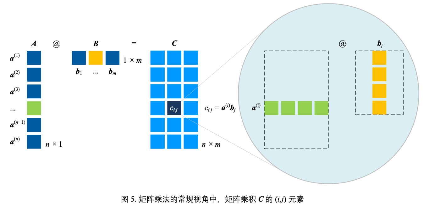
这是最基本、最微观的视角。我们将矩阵 $W$ 看作是一个 $3 \times 6$ 的数字网格。结果向量 $y$ 中的每一个元素 $y_j$,都是通过将向量 $x$ 的每个元素与其在矩阵 $W$ 中对应列的每个元素相乘,然后将结果相加得到的。
简单来说,结果向量 $y$ 的第 $j$ 个元素,是向量 $x$ 与矩阵 $W$ 的第 $j$ 列的点积。
设 $y = \begin{bmatrix} y_1 & y_2 & y_3 & y_4 & y_5 & y_6 \end{bmatrix}$。其计算过程如下:
$$ y_1 = x_1 w_{11} + x_2 w_{21} + x_3 w_{31} \\\\ y_2 = x_1 w_{12} + x_2 w_{22} + x_3 w_{32} \\\\ y_3 = x_1 w_{13} + x_2 w_{23} + x_3 w_{33} \\\\ y_4 = x_1 w_{14} + x_2 w_{24} + x_3 w_{34} \\\\ y_5 = x_1 w_{15} + x_2 w_{25} + x_3 w_{35} \\\\ y_6 = x_1 w_{16} + x_2 w_{26} + x_3 w_{36} $$我们可以将其写成一个更紧凑的求和公式:
$$y_j = \sum_{i=1}^{3} x_i w_{ij} \quad \text{for } j=1, 2, \dots, 6$$角度二:将 W 视为由 3 个行向量组成
在这个视角下,我们将矩阵 $W$ 看作是由三个形状为 $(1, 6)$ 的行向量 $w_{\text{row1}}, w_{\text{row2}}, w_{\text{row3}}$ 堆叠而成的。
$$ W = \begin{bmatrix} \text{--- } w_{\text{row1}} \text{ ---} \\\\ \text{--- } w_{\text{row2}} \text{ ---} \\\\ \text{--- } w_{\text{row3}} \text{ ---} \end{bmatrix} $$其中:
- $w_{\text{row1}} = \begin{bmatrix} w_{11} & w_{12} & w_{13} & w_{14} & w_{15} & w_{16} \end{bmatrix}$
- $w_{\text{row2}} = \begin{bmatrix} w_{21} & w_{22} & w_{23} & w_{24} & w_{25} & w_{26} \end{bmatrix}$
- $w_{\text{row3}} = \begin{bmatrix} w_{31} & w_{32} & w_{33} & w_{34} & w_{35} & w_{36} \end{bmatrix}$
向量 $x = \begin{bmatrix} x_1 & x_2 & x_3 \end{bmatrix}$ 中的元素可以被看作是这些行向量的“权重”或“系数”。整个乘法运算 $xW$ 的结果是 $W$ 的行向量的一个线性组合 (Linear Combination)。
$$y = x_1 \cdot w_{\text{row1}} + x_2 \cdot w_{\text{row2}} + x_3 \cdot w_{\text{row3}}$$这个运算将三个 $(1, 6)$ 的行向量组合成一个最终的 $(1, 6)$ 向量。这个视角在理解神经网络中的线性层时特别有用,其中输入向量 $x$ 的每个元素都在“激活”或“缩放”权重矩阵中的相应行。
当你的目标是理解输入向量中的某一个特定分量对整个输出结果有什么影响的时候,行向量视角是最好的。
- 提问方式:“输入
x的第i个元素x_i对最终结果y做了什么贡献?” - 回答:它把矩阵
W的第i行进行了缩放,然后加总到最终结果y中。 - 公式:$y = \sum x_i \cdot W_{row_i}$
这个视角非常适合用来正向推演一个特定输入的影响力。
角度三:将 W 视为由 6 个列向量组成
在这个视角下,我们将矩阵 $W$ 看作是由六个形状为 $(3, 1)$ 的列向量 $w_{\text{col1}}, w_{\text{col2}}, \dots, w_{\text{col6}}$ 并列组成的。
$$ W = \begin{bmatrix} \vert & \vert & & \vert \\\\ w_{\text{col1}} & w_{\text{col2}} & \dots & w_{\text{col6}} \\\\ \vert & \vert & & \vert \end{bmatrix} $$其中:
$$ w_{\text{col1}} = \begin{bmatrix} w_{11} \\ w_{21} \\ w_{31} \end{bmatrix}, \quad w_{\text{col2}} = \begin{bmatrix} w_{12} \\ w_{22} \\ w_{32} \end{bmatrix}, \quad \dots, \quad w_{\text{col6}} = \begin{bmatrix} w_{16} \\ w_{26} \\ w_{36} \end{bmatrix} $$从这个角度看,$xW$ 的运算过程是行向量 $x$ 与矩阵 $W$ 的每一个列向量分别进行点积 (Dot Product) 运算。每次点积的结果都是一个标量(一个数字),这些标量共同构成了最终的输出行向量 $y$。
$$ y = \begin{bmatrix} x \cdot w_{\text{col1}} & x \cdot w_{\text{col2}} & x \cdot w_{\text{col3}} & x \cdot w_{\text{col4}} & x \cdot w_{\text{col5}} & x \cdot w_{\text{col6}} \end{bmatrix} $$这与角度一中的计算是完全一致的,但思考方式有所不同。它强调了输出向量的每个分量是如何独立地由输入向量和矩阵的相应列决定的。这种视角在理解投影等几何变换时非常直观。
当你的目标是理解输出向量中的某一个特定分量是如何产生的时候,列向量视角是最好的。
- 提问方式:“最终结果
y的第j个元素y_j是从哪里来的?” - 回答:它来自于整个输入向量
x与矩阵W的第j列的点积。 - 公式:$y_j = x \cdot W_{col_j}$
这个视角非常适合用来反向追溯一个特定输出的来源。
Matmul
主要研究 C = A @ B,其中 A 和 B 都为矩阵
- A 的形状为
n x D - B 的形状为
D x m - C 的形状为
n x m
标量积展开
- A 看做行向量集合
- n 个行向量,每个向量形状为
1 x D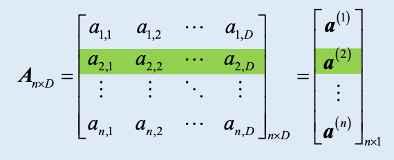
- n 个行向量,每个向量形状为
- B 看做列向量集合
- m 个列向量,每个向量形状为
D x 1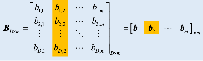
- m 个列向量,每个向量形状为
$\boldsymbol{C} = \boldsymbol{A}\boldsymbol{B} = \begin{bmatrix} \boldsymbol{a}^{(1)} \\ \boldsymbol{a}^{(2)} \\ \vdots \\ \boldsymbol{a}^{(n)} \end{bmatrix}_{n \times 1} \begin{bmatrix} \boldsymbol{b}_{1} & \boldsymbol{b}_{2} & \cdots & \boldsymbol{b}_{m} \end{bmatrix}_{1 \times m} = \begin{bmatrix} \boldsymbol{a}^{(1)}\boldsymbol{b}_{1} & \boldsymbol{a}^{(1)}\boldsymbol{b}_{2} & \cdots & \boldsymbol{a}^{(1)}\boldsymbol{b}_{m} \\ \boldsymbol{a}^{(2)}\boldsymbol{b}_{1} & \boldsymbol{a}^{(2)}\boldsymbol{b}_{2} & \cdots & \boldsymbol{a}^{(2)}\boldsymbol{b}_{m} \\ \vdots & \vdots & \ddots & \vdots \\ \boldsymbol{a}^{(n)}\boldsymbol{b}_{1} & \boldsymbol{a}^{(n)}\boldsymbol{b}_{2} & \cdots & \boldsymbol{a}^{(n)}\boldsymbol{b}_{m} \end{bmatrix}_{n \times m}$
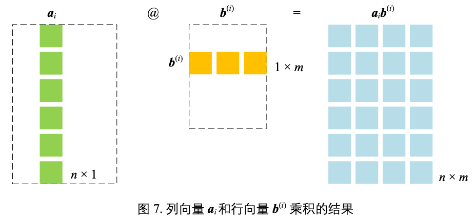
外积展开
- A 看做列向量集合
- D 个列向量,每个向量形状为
n x 1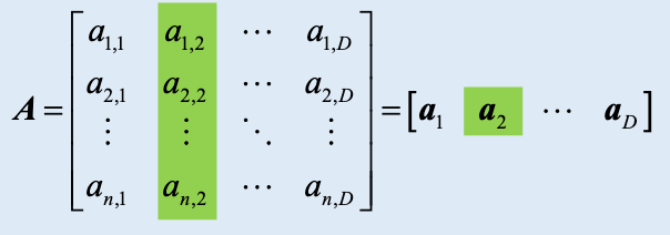
- D 个列向量,每个向量形状为
- B 看做行向量集合
- D 个行向量,每个向量形状为
1 x m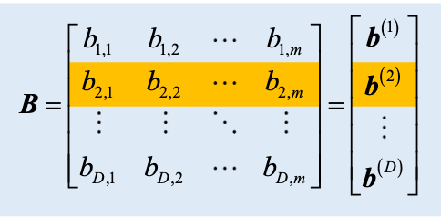
- D 个行向量,每个向量形状为
$\boldsymbol{C} = \boldsymbol{A}\boldsymbol{B} = \begin{bmatrix} \boldsymbol{a}_{1} & \boldsymbol{a}_{2} & \cdots & \boldsymbol{a}_{D} \end{bmatrix}_{1 \times D} \begin{bmatrix} b^{(1)} \\ b^{(2)} \\ \vdots \\ b^{(D)} \end{bmatrix}_{D \times 1} = \boldsymbol{a}_{1}b^{(1)} + \boldsymbol{a}_{2}b^{(2)} + \cdots + \boldsymbol{a}_{D}b^{(D)} = \sum_{i=1}^{D} \boldsymbol{a}_{i}b^{(i)}$
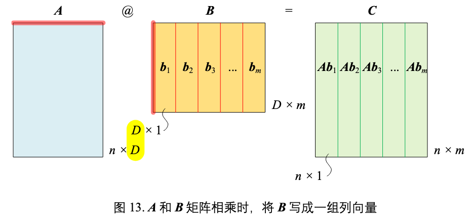
B 切为列向量
A 和 B 矩阵相乘时,将 B 分割成列向量,这样 AB 结果为:
$\boldsymbol{C} = \boldsymbol{A}\boldsymbol{B} = \boldsymbol{A}\begin{bmatrix} \boldsymbol{b}_{1} & \boldsymbol{b}_{2} & \cdots & \boldsymbol{b}_{m} \end{bmatrix} = \begin{bmatrix} \boldsymbol{A}\boldsymbol{b}_{1} & \boldsymbol{A}\boldsymbol{b}_{2} & \cdots & \boldsymbol{A}\boldsymbol{b}_{m} \end{bmatrix}$
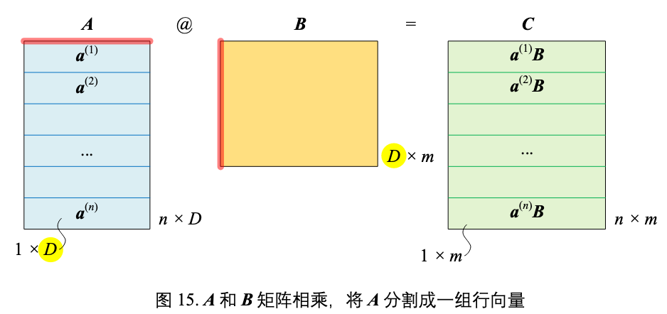
A 切为行向量
- 将 A 分割成一组行向量
- n 个行向量,每个向量形状为
1 x D
- n 个行向量,每个向量形状为
- B 矩阵形状为
D x m
乘积 AB 结果为:
$\boldsymbol{C} = \boldsymbol{A}\boldsymbol{B} = \begin{bmatrix} \boldsymbol{a}^{(1)} \\ \boldsymbol{a}^{(2)} \\ \vdots \\ \boldsymbol{a}^{(n)} \end{bmatrix}_{n \times 1} @ \boldsymbol{B} = \begin{bmatrix} \boldsymbol{a}^{(1)}\boldsymbol{B} \\ \boldsymbol{a}^{(2)}\boldsymbol{B} \\ \vdots \\ \boldsymbol{a}^{(n)}\boldsymbol{B} \end{bmatrix}_{n \times 1}$
矩阵分块
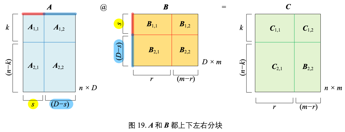
A 和 B 都上下左右分块,乘积 AB 结果为:
$\mathbf{A}\mathbf{B} = \begin{bmatrix} \mathbf{A}_{1,1} & \mathbf{A}_{1,2} \\ \mathbf{A}_{2,1} & \mathbf{A}_{2,2} \end{bmatrix} \begin{bmatrix} \mathbf{B}_{1,1} & \mathbf{B}_{1,2} \\ \mathbf{B}_{2,1} & \mathbf{B}_{2,2} \end{bmatrix} = \begin{bmatrix} \mathbf{A}_{1,1}\mathbf{B}_{1,1} + \mathbf{A}_{1,2}\mathbf{B}_{2,1} & \mathbf{A}_{1,1}\mathbf{B}_{1,2} + \mathbf{A}_{1,2}\mathbf{B}_{2,2} \\ \mathbf{A}_{2,1}\mathbf{B}_{1,1} + \mathbf{A}_{2,2}\mathbf{B}_{2,1} & \mathbf{A}_{2,1}\mathbf{B}_{1,2} + \mathbf{A}_{2,2}\mathbf{B}_{2,2} \end{bmatrix}$
LLM Structure
MLP layer
MLP 包含三个部分:
- 上投影:$W_{up} \in \mathbb{R}^{d \times 4d}$
- 激活函数
- 下投影:$W_{down} \in \mathbb{R}^{4d \times d}$
一个完整的计算流程是
input x: (1, d_model)
↓
h = x @ W_up (1, d_model) @ (d_model, d_ffn) = (1, d_ffn)
↓
a = activation(h): (1, d_ffn)
↓
y = a @ W_down (1, d_ffn) @ (d_ffn, d_model) = (1, d_model)
在机器学习中,通常用行向量来表示 $x$,这样有两个好处:
- 批处理的自然扩展
- 单个样本:
x (1×d) → xW (1×d_out) - 批处理:
X (batch×d) → XW (batch×d_out)
- 直观的数据组织
- 每一行代表一个样本
- 每一列代表一个特征
- 符合数据科学中"样本×特征"的直觉
在 MLP 中,有一个关键洞察是:W_up 的第 i 列和 W_down 的第 i 行是联系在一起的:
Note that in the FFN layer, the usage of the ith column from the up projection and the ith row from the down projection coincides with the activation of the ith intermediate neuron.
- 中间激活值
h_i通过x与W_up的第i列计算得到。 - 然后,这个激活值
h_i作为权重,去“激活”或“调用”W_down的第i行,将其按比例贡献给最终的输出y。
Parallelism of FFN
代码:
# English comments are used as requested in user instructions.
import numpy as np


# Let's define the SiLU activation function, as it's central to the FFN block.
# SiLU(x) = x * sigmoid(x)
def sigmoid(x):
    return 1 / (1 + np.exp(-x))


def silu(x):
    return x * sigmoid(x)


# --- 1. Setup Simulation Parameters ---

# Number of devices (e.g., GPUs) to simulate for tensor parallelism.
num_devices = 4

# Define the dimensions of the model and input.
# For demonstration, these values are smaller than in a real model like Llama.
batch_size = 8
hidden_dim = 1024  # Dimension of the input and output 'x'
intermediate_dim = 4096  # The expanded inner dimension of the FFN

# Ensure intermediate_dim is divisible by num_devices for clean splitting.
assert intermediate_dim % num_devices == 0, (
    "intermediate_dim must be divisible by num_devices"
)

print(f"Simulating FFN parallelization across {num_devices} devices.")
print(
    f"Dimensions: Batch={batch_size}, Hidden={hidden_dim}, Intermediate={intermediate_dim}\n"
)

# --- 2. Initialize Input and Weights (Ground Truth) ---

# Create a random input tensor 'x'.
# In a real scenario, this comes from the previous Attention Block.
np.random.seed(42)
x = np.random.randn(batch_size, hidden_dim)

# Initialize the three weight matrices for the entire FFN block.
# These are the "unsplit" weights that would exist on a single device.
W_gate = np.random.randn(hidden_dim, intermediate_dim)
W_up = np.random.randn(hidden_dim, intermediate_dim)
W_down = np.random.randn(intermediate_dim, hidden_dim)


# --- 3. Baseline: Single-Device FFN Calculation ---
# This is our ground truth to verify the parallelized version.

print("--- Running Baseline Calculation (Single Device) ---")

# The formula is: Output = W_down(SiLU(W_gate(x)) * W_up(x))
gate_proj = x @ W_gate
up_proj = x @ W_up
# Element-wise multiplication
fused_hidden = silu(gate_proj) * up_proj
single_device_output = fused_hidden @ W_down

print(f"Shape of single_device_output: {single_device_output.shape}\n")


# --- 4. Parallelized FFN Calculation ---
# This simulates the process across multiple devices.

print("--- Running Parallelized Calculation (Simulated Multi-Device) ---")

# Step 0: Split the weights across the devices.
# W_gate and W_up are split by COLUMNS (axis=1). This is "Column Parallelism".
W_gate_shards = np.array_split(W_gate, num_devices, axis=1)
W_up_shards = np.array_split(W_up, num_devices, axis=1)

# W_down is split by ROWS (axis=0). This is "Row Parallelism".
W_down_shards = np.array_split(W_down, num_devices, axis=0)

print(f"Original W_gate shape: {W_gate.shape}")
print(f"Split W_gate_shard[0] shape: {W_gate_shards[0].shape}")
print(f"Original W_down shape: {W_down.shape}")
print(f"Split W_down_shard[0] shape: {W_down_shards[0].shape}\n")


# This list will hold the partial output from each device before the final communication.
partial_outputs = []

# --- Loop to simulate computation on each device ---
for i in range(num_devices):
    print(f"-> Simulating computation on Device {i}...")

    # The full input 'x' is available on every device (broadcast).
    device_input = x

    # Get the weight shards for this specific device.
    w_gate_i = W_gate_shards[i]
    w_up_i = W_up_shards[i]
    w_down_i = W_down_shards[i]

    # Step 1 & 2: Column and Row Parallelism Calculation
    # Each device performs its computation independently. NO communication is needed yet.

    # Column Parallelism part:
    # Each device computes a slice of the gate and up projections.
    gate_proj_i = device_input @ w_gate_i
    up_proj_i = device_input @ w_up_i

    # Local activation and element-wise multiplication.
    fused_hidden_i = silu(gate_proj_i) * up_proj_i

    # Row Parallelism part:
    # The intermediate result is multiplied by the corresponding ROW-split part of W_down.
    # The result is a partial output that has the final correct dimension.
    output_i = fused_hidden_i @ w_down_i

    print(f"   Shape of partial output on Device {i}: {output_i.shape}")

    # Store the partial result.
    partial_outputs.append(output_i)

print("\n--- Step 3: All-Reduce Aggregation ---")

# In a real system, this would be a single, highly optimized MPI or NCCL call.
# The all_reduce operation sums the tensors from all devices element-wise
# and makes the final result available on all devices.
# Here, we simply sum the partial results from our list.
parallel_device_output = sum(partial_outputs)

print(f"Shape of aggregated parallel_device_output: {parallel_device_output.shape}\n")


# --- 5. Verification ---
# Compare the output from the single-device calculation with the parallelized one.

print("--- Verification ---")
are_close = np.allclose(single_device_output, parallel_device_output, atol=1e-6)
print(
    f"Do the results from single-device and parallelized computation match? -> {are_close}"
)

if are_close:
    print(
        "✅ Success! The parallel FFN implementation correctly reproduces the original output."
    )
else:
    print("❌ Failure! The outputs do not match.")
- 输入 $X\in\mathbb{R}^{B\times H}$(batch $B$、hidden 维度 $H$)
- 三个权重:
- $W_{\text{gate}}\in\mathbb{R}^{H\times I}$
- $W_{\text{up}}\in\mathbb{R}^{H\times I}$
- $W_{\text{down}}\in\mathbb{R}^{I\times H}$
- 中间量:
- $G = X W_{\text{gate}}\in\mathbb{R}^{B\times I}$
- $U = X W_{\text{up}}\in\mathbb{R}^{B\times I}$
- $H_{\text{fused}}=\text{SiLU}(G)\odot U\in\mathbb{R}^{B\times I}$
- 输出 $Y = H_{\text{fused}}\, W_{\text{down}}\in\mathbb{R}^{B\times H}$
代码的并行拆分是:
对 $W_{\text{gate}}, W_{\text{up}}$ 做按列切分(column-parallel),对 $W_{\text{down}}$ 做按行切分(row-parallel)。设设备数为 $D$,把中间维 $I$ 均分为 $I=I_1+\cdots+I_D$。对应地:
$$ W_{\text{gate}} = \big[ W_{\text{gate}}^{(1)}\;|\;\cdots\;|\;W_{\text{gate}}^{(D)} \big],\quad W_{\text{up}} = \big[ W_{\text{up}}^{(1)}\; |\;\cdots\;|\;W_{\text{up}}^{(D)} \big], $$其中 $W_{\text{gate}}^{(i)},W_{\text{up}}^{(i)}\in\mathbb{R}^{H\times I_i}$;
$$ W_{\text{down}} = \begin{bmatrix} W_{\text{down}}^{(1)}\\ \vdots\\ W_{\text{down}}^{(D)} \end{bmatrix},\quad W_{\text{down}}^{(i)}\in\mathbb{R}^{I_i\times H}. $$列并行拆分
矩阵乘法按列块的恒等式:
$$ X W_{\text{gate}}=\big[\,X W_{\text{gate}}^{(1)}\;\big|\;\cdots\;\big|\;X W_{\text{gate}}^{(D)}\,\big], $$因此每个设备 $i$ 都能独立得到本地的投影片段
$$ G^{(i)} = X W_{\text{gate}}^{(i)} \in \mathbb{R}^{B\times I_i},\quad U^{(i)} = X W_{\text{up}}^{(i)} \in \mathbb{R}^{B\times I_i}. $$由于 $\text{SiLU}$ 与“逐元素乘” $\odot$ 都是按列独立的逐元素操作,所以每个设备可在本地完成
$$ H_{\text{fused}}^{(i)}=\text{SiLU}(G^{(i)})\odot U^{(i)} \in \mathbb{R}^{B\times I_i} $$而无需和别的设备通信;把所有 $H_{\text{fused}}^{(i)}$ 横向拼起来就得到完整的
$$ H_{\text{fused}}=\big[H_{\text{fused}}^{(1)}\;|\;\cdots\;|\;H_{\text{fused}}^{(D)}\big]\in\mathbb{R}^{B\times I}. $$行并行 + 外积展开
把中间结果按列切成块、把 W_down 权重按行切成块:
$$ H_{\text{fused}}=\big[H^{(1)}\;|\;H^{(2)}\;|\;\cdots\;|\;H^{(D)}\big],\quad W_{\text{down}}=\begin{bmatrix} W^{(1)}\\ W^{(2)}\\ \vdots \\ W^{(D)} \end{bmatrix} $$那么最关键的乘法就是一个非常朴素的块矩阵恒等式:
$$ H_{\text{fused}}\,W_{\text{down}} =\big[H^{(1)}|\cdots|H^{(D)}\big] \begin{bmatrix}W^{(1)}\\ \vdots \\ W^{(D)}\end{bmatrix} =\;H^{(1)}W^{(1)}\;+\;\cdots\;+\;H^{(D)}W^{(D)}. $$所以在列并行结束后,设备之间不用相互通信,正好可以用自己本地的 $H_{fused}^{(i)}$,在本地进行 $H^{(i)}W^{(i)}$ 计算,最后再 allreduce 到一起。
Linear Layer
Linear 层的实现:
def linear(
    x: mx.array,
    w: mx.array,
    bias: mx.array | None = None,
) -> mx.array:
    assert x.shape[-1] == w.shape[-1], "x.shape[-1] != w.shape[-]"
    return x @ w.T + (bias if bias is not None else 0)
所以全连接层的权重矩阵习惯上存储为 (输出维度 × 输入维度)。
Quantization
Per-tensor && Per-group Quantization
- Per-tensor Quantization
- 对一整个张量(Tensor)使用同一套量化参数。一个张量可以理解为一个多维数组,在神经网络中通常指一整层的权重或激活值。
- 一个张量,一套缩放因子和零点
- 精度低,开销低
- Per-group Quantization
- 将一个大张量分割成多个 groups,然后为每一个 group 独立计算并应用一套量化参数。
- 一个张量,多套缩放因子和零点
- 精度高,开销高
Parallelism
KV Cache in TP
这里要明确的是,多头注意力 (Multi-Head Attention) 的本质是: 将输入向量先通过线性变换拆成多个子空间,每个子空间对应一个 head,分别计算注意力分数,最后拼接结果。
多头并未增加新的非线性类型,只是把 softmax 做了 H 次、彼此独立归一化。正是“多个独立归一化”的结构性差异,带来更强表达能力(同一位置可同时“看向”不同位置并对不同通道采取不同的加权策略)。
因此,每个 head 都有自己独立的一组投影矩阵 (W_Q, W_K, W_V)。 对应到 KV Cache:每个 head 会生成一份自己的 Key、Value,并存入缓存。
不同 head 的 KV cache 不会共用,而是按 head 维度单独存放。
比如在下面这段实现中,同一层只使用了一个 cache 对象,看起来像是多个 head 共用了 KV Cache,其实只是 共用一个容器,不共用内容
class MultiHeadAttention(nn.Module):
    def __init__(self, args: ModelArgs):
        super().__init__()
        self.n_embd = args.n_embd
        self.n_head = args.n_head
        self.head_dim = self.n_embd // self.n_head

        self.scale = self.head_dim**-0.5

        # D x 3D (Q, K, V)
        self.c_attn = nn.Linear(self.n_embd, 3 * self.n_embd, bias=True)
        self.c_proj = nn.Linear(self.n_embd, self.n_embd, bias=True)

    def __call__(
        self,
        x: mx.array,
        mask: Optional[mx.array | Literal["causal"]] = None,
        cache: Optional[Any] = None,
    ) -> mx.array:
        N, L, E = x.shape
        H, D = self.n_head, self.head_dim

        assert E == H * D, (
            f"Embedding size {E} must be divisible by number of heads {H}."
        )

        qkv = self.c_attn(x)
        # N x L x E
        q, k, v = mx.split(qkv, 3, axis=-1)

        # N x L x (H * D)
        q = q.reshape(N, L, H, D)
        k = k.reshape(N, L, H, D)
        v = v.reshape(N, L, H, D)

        # multihead attention expects
        # N x H x L x D
        q = q.swapaxes(1, 2)
        k = k.swapaxes(1, 2)
        v = v.swapaxes(1, 2)

        if cache is not None:
            k, v = cache.update_and_fetch(k, v)

        # N x H x L x D
        x = scaled_dot_product_attention(
            q, k, v, scale=self.scale, cache=cache, mask=mask
        )
        # N x L x (H * D)
        x = x.swapaxes(1, 2)
        x = x.reshape(N, L, H * D)
        return self.c_proj(x)
典型实现里,cache 会把传入的 (N, H, L_new, D) 追加到内部维护的 (N, H, L_total, D) 上(沿着 序列维拼接)。head 维不会被合并或相互写入,因此每个 head 的缓存仍是独立切片:k[:, h, :, :] / v[:, h, :, :].
API
Function Calling
- 本地作为 Function Handler, 提供
- Function Description
- Descriptions about when to call this function
- Function Parameters, including the type
- Function Implementation
- Function Description
- Prompt 中包括
- 用户输入
- Function Description
- LLM 根据用户输入,决定是否要调用工具来获取信息
- 否:正常返回
- 是:返回一个
tool_calls(LLM issues a function call)
- 本地收到
tool_calls时,通过 Function Handler 调用对应的 Function,然后返回给 LLM - LLM 结合 Function Call 的结果,生成响应
A practical example
Setup:
uv venv
uv pip install openai
import json
import os

from openai import OpenAI

# --- 1. Setup (Modified Section) ---
# Read API key and optional Base URL from environment variables.
# This is a best practice for security and flexibility, allowing you
# to use different API providers or proxies without changing the code.
api_key = "xxxx"
base_url = "https://openrouter.ai/api/v1"

# Check if the API key is provided, which is essential.
if not api_key:
    print("Error: The OPENAI_API_KEY environment variable is not set.")
    exit()

# Initialize the OpenAI client.
# The `base_url` parameter is optional. If it's None (not set as an env var),
# the client will default to OpenAI's official API endpoint.
try:
    client = OpenAI(
        api_key=api_key,
        base_url=base_url,
    )
    print(f"--- Client initialized. Using Base URL: {client.base_url} ---")
except Exception as e:
    print(f"Error initializing OpenAI client: {e}")
    exit()


# --- 2. Define the Tool (Your Python Function) ---
# This part remains unchanged.
def get_current_weather(location, unit="celsius"):
    """
    Get the current weather in a given location.

    Args:
        location (str): The city and state, e.g., "San Francisco, CA".
        unit (str): The unit for the temperature, can be "celsius" or "fahrenheit".

    Returns:
        str: A JSON string with weather information.
    """
    print(f"--- Executing 'get_current_weather' for {location} ---")
    if "tokyo" in location.lower():
        return json.dumps(
            {
                "location": "Tokyo",
                "temperature": "15",
                "unit": unit,
                "forecast": "rainy",
            }
        )
    elif "san francisco" in location.lower():
        return json.dumps(
            {
                "location": "San Francisco",
                "temperature": "22",
                "unit": unit,
                "forecast": "sunny",
            }
        )
    elif "paris" in location.lower():
        return json.dumps(
            {
                "location": "Paris",
                "temperature": "18",
                "unit": unit,
                "forecast": "cloudy",
            }
        )
    else:
        return json.dumps({"location": location, "temperature": "unknown"})


# --- 3. Main Conversation Loop ---
# This part remains unchanged.
def run_conversation():
    messages = [
        {
            "role": "user",
            "content": "What's the weather like in San Francisco and Tokyo?",
        }
    ]

    tools = [
        {
            "type": "function",
            "function": {
                "name": "get_current_weather",
                "description": "Get the current weather in a given location",
                "parameters": {
                    "type": "object",
                    "properties": {
                        "location": {
                            "type": "string",
                            "description": "The city and state, e.g., San Francisco, CA",
                        },
                        "unit": {"type": "string", "enum": ["celsius", "fahrenheit"]},
                    },
                    "required": ["location"],
                },
            },
        }
    ]

    print("\n--- Step 1: First API Call (Model decides to use a tool) ---")
    response = client.chat.completions.create(
        model="openai/gpt-4.1",
        messages=messages,
        tools=tools,
        tool_choice="auto",
    )

    response_message = response.choices[0].message
    print("\n[Model's First Response - Tool Call Request]")
    print(response_message)

    tool_calls = response_message.tool_calls
    if tool_calls:
        messages.append(response_message)
        available_functions = {"get_current_weather": get_current_weather}

        for tool_call in tool_calls:
            function_name = tool_call.function.name
            function_to_call = available_functions[function_name]
            function_args = json.loads(tool_call.function.arguments)
            function_response = function_to_call(**function_args)
            messages.append(
                {
                    "tool_call_id": tool_call.id,
                    "role": "tool",
                    "name": function_name,
                    "content": function_response,
                }
            )

        print(
            "\n--- Step 2: Second API Call (Sending tool results back to the model) ---"
        )
        second_response = client.chat.completions.create(
            model="gpt-4o",
            messages=messages,
        )

        final_response = second_response.choices[0].message
        print("\n--- Step 3: Final Answer from Model ---")
        print(final_response.content)
    else:
        print("\n--- Final Answer from Model (No Tool Call) ---")
        print(response_message.content)


# Run the main function
if __name__ == "__main__":
    run_conversation()
MCP
MCP协议主要解决大模型需要访问外部资源和工具的问题,包括:
- 资源访问:文件系统、数据库、API等
- 工具调用:执行特定功能的外部工具
- 上下文管理:安全地管理和传递上下文信息
主要特点:
- 标准化接口:提供统一的协议规范,让不同的AI应用可以无缝集成各种外部服务。
- 安全性:内置权限管理和访问控制机制,确保数据访问的安全性。
- 可扩展性:支持插件式架构,开发者可以轻松添加新的资源类型和工具。
工作原理:
- 连接建立:AI应用通过MCP协议连接到外部资源服务器
- 能力协商:双方协商支持的功能和权限范围
- 请求处理:AI应用发送标准化请求,服务器返回结构化响应
- 上下文同步:维护会话状态和上下文信息
MCP 协议和 Function Calling 都能让大模型调用外部功能。
传统 Function Calling:
AI 应用 ←→ Function Handler

MCP 协议:
AI 应用 ←→ MCP 客户端 ←→ MCP 服务器
MCP 可以看做是高级版的 Function Call
- MCP Server 在云端提供 Function Call
- MCP Client 在本地提供更完善的错误处理和重试机制
Boundwidth
“设备的内存带宽”通常指的是算力核心(CPU/GPU/加速器的计算单元)⇄外部设备内存(DDR/GDDR/HBM)之间,经过内存控制器到片上缓存/寄存器的有效数据吞吐能力。
内存带宽(这里的“内存”):指 设备外部 DRAM(HBM/GDDR/DDR)⇄ 芯片内部(L2/L1/寄存器/SM) 的数据通道的可持续吞吐。
不等于 主机内存⇄显存(PCIe/NVLink 的对外带宽),也不等于磁盘⇄内存(IO 带宽)。
真实执行里存在分层:HBM ⇄ L2 ⇄ SM 寄存器/共享内存。所谓“带宽瓶颈”,通常指HBM 这一层供数不应求。
显存带宽指的是 显存芯片(GDDR6/HBM 等外部 DRAM) ↔ GPU 芯片内部(内存控制器/L2 缓存/SM 寄存器)之间的最大可持续数据传输速率
在大模型推理解码的“内圈”里,关键数据(权重、KV cache、激活)已经常驻在 GPU 的显存(HBM/GDDR)里,计算单元每一步都在从显存拉这些数据。 因此瓶颈通常是显存⇄GPU 核心的带宽(显存带宽),不是主机内存⇄显存(PCIe/NVLink-H2D)的带宽。主机内存到显存的拷贝要么只发生在启动/换模型时,要么量级很小(输入输出token),被摊薄掉了。