PyTorch Notes
PyTorch 常用张量操作(高级索引、einsum、scatter、gather 等)、monkey patching,以及从前向传播、DataLoader 到训练循环和模型保存的基础流程。
- Doc no.
- KKZ-TN-122
- Date
- 2026-01-15
- GMT day
- 2026:015
- Est. read
- 15 min
01Tensor Operations#
1.1clamp#
torch.clamp(或 Tensor 的实例方法 .clamp)是 PyTorch 中用于数值截断(clipping)的常用操作。它的主要作用是将输入张量(Tensor)中的所有元素限制在一个指定的范围内 。
Example:
import torch

# Initialize a tensor with values ranging from -10 to 10
data = torch.tensor([-10.0, -5.0, 0.5, 5.0, 10.0])

print(f"Original: {data}")

# 1. Clamp between a min and max range [-1, 1]
# Values < -1 become -1; Values > 1 become 1
clamped_both = data.clamp(min=-1.0, max=1.0)
print(f"Range [-1, 1]: {clamped_both}")

# 2. Clamp with only a lower bound (min=-2)
# Values < -2 become -2; No upper limit
clamped_min = data.clamp(min=-2.0)
print(f"Min -2 only: {clamped_min}")

# 3. Clamp with only an upper bound (max=3)
# Values > 3 become 3; No lower limit
clamped_max = data.clamp(max=3.0)
print(f"Max 3 only: {clamped_max}")1.2Advanced Indexing#
x[y] 是 PyTorch(以及 NumPy)中非常强大且灵活的**高级索引(Advanced Indexing)**语法
主要分为两种情况:
- y 是整数张量 (LongTensor/IntTensor):这叫整数数组索引(就像查字典)。
- y 是布尔张量 (BoolTensor):这叫掩码索引(就像用筛子过滤)。
y 为整数张量#
# x 是一个 3x4 的矩阵
x = torch.tensor([
    [1, 1, 1, 1], # row 0
    [2, 2, 2, 2], # row 1
    [3, 3, 3, 3]  # row 2
])

# y 是想取的行号
y = torch.tensor([0, 2])

print(x[y])
# 意思:取出第0行和第2行,组成新张量
# Output:
# tensor([[1, 1, 1, 1],
#         [3, 3, 3, 3]])
当 y 是多维时,行为比较复杂:
假设:x 的形状是 (D0, D1, D2)y 的形状是 (M, N) (且 y 中的数值都在 0 ~ D0-1 之间)那么 x[y] 的结果形状将是:
- 前两维:完全继承自 y 的形状 (M, N)。
- 后两维:继承自 x 剩余的维度 (D1, D2)(因为你只是指定了第 0 维取谁,后面的维度是被整个搬过来的)。
可以认为是只会取第 0 维的数据 可以把 y 想象成一个**“模具”或“容器”**,x 是填充材料。PyTorch 会按照 y 的形状造出一个新张量,然后把 y 里每个整数对应的 x 中的数据填进去。
import torch

# x: 词表,有5个词,每个词向量长度为4
x = torch.randn(5, 4)

# y: 两个句子,每个句子3个词的索引
y = torch.tensor([
    [1, 2, 4],  # Sentence 1: word 1, word 2, word 4
    [0, 0, 3]   # Sentence 2: word 0, word 0, word 3
])

out = x[y]

# 结果形状解析:
# y.shape = [2, 3]
# x.shape = [5, 4] (我们在第0维索引,剩下了第1维)
# Result  = [2, 3] + [4] = [2, 3, 4]

print("x shape:", x.shape)
print("y shape:", y.shape)
print("Result shape:", out.shape)
# torch.Size([2, 3, 4])
# 解释:2个句子,每个句子3个词,每个词是4维向量。x[y] 中 y 是“模具”: 结果先继承 y 的形状 , 每个格子再整行填入 x[y[i, j]], 于是末尾补上 x 剩下的维度 ; 颜色标出每一行来自 x 的哪一行y 为布尔值#
y 是一个筛子(Mask)。 y 必须和 x 形状相同(或者可广播)。y 中为 True 的位置,对应的 x 的值会被保留;为 False 的会被丢弃。
- 核心逻辑:只保留满足条件的元素。
- 形状变化:结果通常会被展平(Flatten)为一维。因为计算机无法预知有多少个 True,所以没法保持原来的二维或三维矩形结构,只能把选出来的数排成一条线
import torch

x = torch.tensor([
    [1, 6, 3],
    [8, 2, 9]
])

# 生成一个布尔张量 y (Mask)
# y 会变成 [[False, True, False], [True, False, True]]
y = x > 5

print("Mask:\n", y)

# 使用掩码索引
result = x[y]

print("Result:", result)
# Output: tensor([6, 8, 9])
# 注意:结果变成 1D 了!因为原来矩阵里大于5的位置并不构成一个矩形。
x 和 y 的维度可以不同,只需要前面的维度对齐即可
假设:
- x 的形状:
- y 的形状: (必须与 x 的前两维形状完全匹配)
处理流程如下:
- 对齐: y 覆盖在 x 的前两个维度上。
- 筛选: 只有 y 中为 True 的位置 (i, j) 会被选中。
- 提取: 对于每个被选中的位置 (i, j),
x[i, j, :]这一整条数据(长度为 的向量)被拿出来。 - 拍平堆叠: 因为 True 的位置是不规则的,无法保持 的矩阵结构,所以所有被选中的向量会被堆叠成一个新的二维列表。
最终形状:
其中 是 y 中 True 的总个数。
import torch

# 1. 创建数据 x (3D)
# 假设是 2个样本,每个样本3个像素,每个像素有4个特征(RGBA)
# Shape: (2, 3, 4)
x = torch.tensor([
    # Sample 0
    [[1, 1, 1, 1], [2, 2, 2, 2], [3, 3, 3, 3]],
    # Sample 1
    [[4, 4, 4, 4], [5, 5, 5, 5], [6, 6, 6, 6]]
])

# 2. 创建掩码 y (2D)
# Shape: (2, 3) - 必须匹配 x 的前两维
y = torch.tensor([
    [True,  False, True ], # Sample 0: 选第1个和第3个像素
    [False, True,  False]  # Sample 1: 选第2个像素
])

# 3. 执行索引
result = x[y]

print("x shape:", x.shape)       # [2, 3, 4]
print("y shape:", y.shape)       # [2, 3]
print("True count in y:", y.sum()) # 3 个 True

print("\nResult shape:", result.shape)
# Expect: [3, 4] -> (True的总数, 剩余的最后一维)

print("Result data:\n", result)
# Output:
# tensor([[1, 1, 1, 1],  <- 来自 (0,0)
#         [3, 3, 3, 3],  <- 来自 (0,2)
# [5, 5, 5, 5]]) <- 来自 (1,1)x 的前两维上: 每个 True 位置取出一整条长度为 4 的向量, 按行优先顺序堆叠成 1.3repeat#
理解为贴瓷砖
torch.repeat 是一个用于复制张量数据的操作
函数签名: Tensor.repeat(*sizes)
*sizes(int…): 你希望沿着每个维度重复多少次。- 返回值: 一个全新的张量,其数据在内存中是物理复制的。
repeat 的参数数量必须大于等于输入张量的维度数。 假设你有一个形状为 (H, W) 的 2D 张量,你调用 .repeat(a, b):
- 新的行数变成了 。
- 新的列数变成了 。
import torch

# A small 2x2 matrix
x = torch.tensor([
    [1, 2],
    [3, 4]
])

# Repeat 2 times vertically, 3 times horizontally
y = x.repeat(2, 3)

print("Original Shape:", x.shape) # [2, 2]
print("New Shape     :", y.shape) # [2*2, 2*3] = [4, 6]
print("Result:\n", y)

# Output:
# tensor([[1, 2, 1, 2, 1, 2],  <-- Top-Left block repeated 3 times across
#         [3, 4, 3, 4, 3, 4],
#         [1, 2, 1, 2, 1, 2],  <-- The whole row block repeated 2 times down
#         [3, 4, 3, 4, 3, 4]])
如果传入的参数个数多于原张量的维度,PyTorch 会自动在前面增加维度(unsqueezing),然后再复制。
import torch

x = torch.tensor([1, 2, 3]) # Shape: [3]

# unsqueeze to (1, 3) first

# Repeat 4 times along a NEW dimension (dim 0),
# and 1 time along the original dimension (dim 1)
y = x.repeat(4, 1)

print("Shape:", y.shape)
print("Result:\n", y)

# Output:
# Shape: torch.Size([4, 3])
# Result:
#  tensor([[1, 2, 3],
#          [1, 2, 3],
#          [1, 2, 3],
#          [1, 2, 3]])
# Explanation: It effectively stacked 4 copies of the vector.维度对齐#
PyTorch 在处理维度不匹配时,总是遵循从右向左对齐的原则。
假设你有一个 1D 向量 Shape=[2],但你传入了两个参数 repeat(3, 2),意图把它当成 2D 矩阵处理。
PyTorch 会这样思考:
- 目标指令是 2 个维度:(dim0, dim1)。
- 现有数据只有 1 个维度。
- 对齐:把现有的那个维度对应到最右边(dim1)。
补位:前面的空位(dim0)自动补 1。
import torch

# 1. 原始数据:1D 向量
x = torch.tensor([10, 20])
# Shape: [2]
# 样子: [10, 20]

# 2. 调用 repeat(3, 1)
# 参数有两个 (3, 1),原数据只有一维。
# 于是 PyTorch 自动把它变成了 [[10, 20]] (Shape: [1, 2])

y = x.repeat(3, 1)

# 3. 执行复制
# 第一维重复 3 次:意味着有 3 行。
# 第二维重复 1 次:意味着列数不变。

print(y)
# Output:
# tensor([[10, 20],
#         [10, 20],
#         [10, 20]])
# Shape: [3, 2]repeat 是“贴瓷砖”: 整块张量按各维的次数物理复制; 参数比维度多时, 先把形状右对齐, 左侧补 1 再复制1.4torch.einsum#
超级好用
torch.einsum:爱因斯坦求和约定,Einstein Summation
感觉根本不用介绍,代码一看就懂
import torch

A = torch.randn(3, 5) # i=3, k=5
B = torch.randn(5, 4) # k=5, j=4

# 传统写法
res_traditional = torch.matmul(A, B)

# Einsum 写法
# i: 3, k: 5, j: 4
res_einsum = torch.einsum('ik, kj -> ij', A, B)

print(torch.allclose(res_traditional, res_einsum)) # True


batch_size = 10
A = torch.randn(batch_size, 3, 5) # b i k
B = torch.randn(batch_size, 5, 4) # b k j

res_traditional = torch.bmm(A, B)

# Einsum 写法 (非常直观:b保留, k消掉)
res_einsum = torch.einsum('bik, bkj -> bij', A, B)

# self-attention
# b: batch, h: heads, i: query_len, j: key_len, d: head_dim
# Q: b h i d
# K: b h j d
# 我们想把 d 消掉 (点积),保留 b h i j
attention_scores = torch.einsum('bhid, bhjd -> bhij', Q, K)einsum 的规则只有一条: 出现在 -> 右边的字母保留, 只出现在输入里的字母先逐项相乘再求和; 左边是 ik, kj -> ij 计算 的一个元素, 右边是 attention 打分中每个字母的去留einsum 简单到我要关心它是否在性能上有取舍
在现代 PyTorch(尤其是 GPU 上运行大张量)中,torch.einsum 的性能通常与手写的优化代码(如 transpose + matmul)相当,甚至在某些复杂的维度变换场景下更好
假设我们要计算 。
手动写法:
torch.matmul(A, B.transpose(-1, -2))- transpose 操作是一个 View 操作(零拷贝,只修改元数据/步长 strides)。
- matmul 接收到这个“看起来转置了”的张量,检测到步长变化,直接调用 cuBLAS 的 GEMM 接口,并告诉 cuBLAS:“读取 B 的时候按转置方式读”。
Einsum 写法:
torch.einsum('ik, jk -> ij', A, B)- einsum 解析发现 k 维度在 B 中需要对齐但顺序不同。
- 它在底层同样构建了指向 A 和 B 的 strided view。
- 它同样调用了 cuBLAS 的 GEMM。
结论:在这个层面上,两者的底层执行路径几乎是一模一样的。
einops#
有一个小问题是,对于 PyTorch 原生的 torch.einsum 来说,每个维度只能用单个英文字母来表示
但是有一个非常流行的第三方库 einops 可以解决这个问题
from einops import rearrange

out = rearrange(x, 'batch channel height width -> batch height width channel')1.5argmax#
函数签名: torch.argmax(input, dim=None, keepdim=False)
- input: 输入张量。
dim (int, 可选): 沿着哪个维度寻找最大值。
- 如果不指定:它会将张量**展平(flatten)**成一维,然后返回整个张量中最大值的索引(一个标量)。
- 如果指定:它会“压缩”掉该维度,返回每一行/列中最大值的索引。
- keepdim (bool): 是否保持输出张量的维度数(Rank)不变。默认为 False。
import torch

# Batch size = 3, Classes = 4
logits = torch.tensor([
    [0.1, 0.8, 0.05, 0.05], # Sample 0: Class 1 is largest
    [0.9, 0.0, 0.1,  0.0 ], # Sample 1: Class 0 is largest
    [0.2, 0.2, 0.5,  0.1 ]  # Sample 2: Class 2 is largest
])

# Find the class index with the highest score along the class dimension (dim=1)
pred_labels = torch.argmax(logits, dim=1)

print("Predicted Labels:", pred_labels)
# Output: tensor([1, 0, 2])
argmax 与 topk 的关系?
- torch.argmax(x, dim=1) 等价于 torch.topk(x, k=1, dim=1).indices.squeeze(1)。
- argmax 是 topk 的特例(只取第 1 名)
1.6topk#
函数签名:torch.topk(input, k, dim=None, largest=True, sorted=True)
它返回一个包含两个张量 tuple:
- values: 前 个数值本身。
- indices: 这些数值在原张量中的原始下标(索引)。
参数:
- k (int): 你想要“前几名”?
- dim (int): 沿着哪个维度寻找。如果不指定,默认为最后一个维度。
- largest (bool): 是否找最大的 topk
import torch

# Batch size = 3, Number of classes = 5
preds = torch.tensor([
    [0.1, 0.9, 0.0, 0.0, 0.0],  # Sample 0: Class 1 is highest
    [0.2, 0.1, 0.4, 0.1, 0.2],  # Sample 1: Class 2 is highest, then 0 or 4
    [0.0, 0.0, 0.1, 0.8, 0.1]   # Sample 2: Class 3 is highest
])

# Find top 2 predictions for each sample (along dim=1, which is the class dimension)
k = 2
top_vals, top_inds = torch.topk(preds, k=k, dim=1)

print("Top 2 Probabilities:\n", top_vals)
print("Top 2 Class Indices:\n", top_inds)

# Output:
# Top 2 Probabilities:
#  tensor([[0.9000, 0.1000],
#          [0.4000, 0.2000],
#          [0.8000, 0.1000]])
#
# Top 2 Class Indices (The predicted labels):
#  tensor([[1, 0],   -> Sample 0 predicts class 1, then class 0
#          [2, 0],   -> Sample 1 predicts class 2, then class 0
# [3, 2]]) -> Sample 2 predicts class 3, then class 2topk(k=2, dim=1) 沿类别维挑出每行最大的两个: values 和 indices 只有 dim=1 变成 , 其余维度不变; indices 的第一列就是 argmax(dim=1)1.7scatter#
scatter 主要用于根据指定的索引将源张量(source)中的值写入到目标张量(self)中
把 src 中的数据,按照 index 给出的位置,填入到 input 中去
函数签名通常为: Tensor.scatter_(dim, index, src, reduce=None)
- dim (int): 指定在哪个维度上进行索引(scatter)。
- index (LongTensor): 索引张量,指示数据应该被放置在哪里。
- src (Tensor or float): 数据源。这里的数值会被填入目标张量。
假设我们有一个 2D 张量,dim=1(按列操作)。对于 src 中的每一个元素 src[i][j],它会被放置在目标张量 input 的以下位置:
行坐标 (i):保持不变(因为 dim=1,行维度是对齐的)。列坐标:由 index[i][j] 的值决定。如果 dim=0,则行坐标由索引决定,列坐标保持不变:
考虑二维的情况,index 和 src 维度相同,所以 index 只能存储在某列的信息,再控制行数相同,就能精确定位
import torch

# Target: 3x5 matrix of zeros
target = torch.zeros(3, 5)

# Source: 3x2 matrix (values to fill)
src = torch.tensor([
    [1.0, 2.0],
    [3.0, 4.0],
    [5.0, 6.0]
])

# Indices: Where to put the values in each row?
# Row 0: put src[0][0] at col 1, src[0][1] at col 3
# Row 1: put src[1][0] at col 0, src[1][1] at col 2
# Row 2: put src[2][0] at col 4, src[2][1] at col 1
index = torch.tensor([
    [1, 3],
    [0, 2],
    [4, 1]
])

target.scatter_(dim=1, index=index, src=src)

print(target)
# Output explanation:
# Row 0: indices are 1 and 3 -> values 1.0 and 2.0 go there.
# Row 1: indices are 0 and 2 -> values 3.0 and 4.0 go there.
# Row 2: indices are 4 and 1 -> values 5.0 and 6.0 go there.

# Result:
# tensor([[0., 1., 0., 2., 0.],
#         [3., 0., 4., 0., 0.],
# [0., 6., 0., 0., 5.]])scatter_(dim=1): src[i][j] 写到 target 的第 行、第 index[i][j] 列; 颜色标出值来自 src 的哪一列, 没被写到的位置保留原值1.8gather#
gather 是从指定位置收集数据
函数签名通常为: torch.gather(input, dim, index)
- input (Tensor): 源张量,我们要从这里拿数据。
- dim (int): 指定在哪个维度上进行索引(gathering)。
- index (LongTensor): 索引张量,告诉 gather 去哪里取值。输出张量的形状将与 index 的形状完全一致。
gather 根据 index 中提供的值,在 input 的 dim 维度上查找对应的数据。假设 dim=1(按列取值),对于输出张量 out 的每一个位置 (i, j),其数值来源于:
行坐标 (i):保持同步(因为 dim=1)。列坐标:由 index[i][j] 指定。也就是说,index 里的值代表“我要去 input 的这一行的第几列拿数据”。
import torch

# Source: 3x3 Matrix
# [[ 1,  2,  3],
#  [ 4,  5,  6],
#  [ 7,  8,  9]]
input_tensor = torch.tensor([
    [1, 2, 3],
    [4, 5, 6],
    [7, 8, 9]
])

# Indices: 3x2 Matrix
# We want to gather 2 values for each of the 3 rows.
# Row 0: take element at index 0 and 2
# Row 1: take element at index 1 and 1
# Row 2: take element at index 2 and 0
index = torch.tensor([
    [0, 2],
    [1, 1],
    [2, 0]
])

output = torch.gather(input_tensor, dim=1, index=index)

print(output)
# Logic breakdown:
# Row 0: input[0][0]=1, input[0][2]=3  -> [1, 3]
# Row 1: input[1][1]=5, input[1][1]=5  -> [5, 5]
# Row 2: input[2][2]=9, input[2][0]=7  -> [9, 7]

# Result:
# tensor([[1, 3],
#         [5, 5],
# [9, 7]])gather(dim=1) 是 scatter 的反方向: out[i][j] 从 input 第 行、第 index[i][j] 列读取; 输出形状与 index 相同, 同一个元素可以被读多次1.9sum#
a = torch.tensor([[1,2,3],[4,5,6]])
print(a.shape) # torch.Size([2, 3])
print(a.sum(0)) # tensor([5, 7, 9])
print(a.sum(1)) # tensor([ 6, 15])sum(dim) 沿指定维度把元素挤压在一起相加, 这一维从形状中消失; keepdim=True 时保留为大小 1指定哪个维度(dim/axis),哪个维度就会被"拍扁"并求和,从而在形状中消失
这是最常用也最容易晕的地方。想象一个 Excel 表格(2行3列),形状是 。
sum(0):消除第 0 维(行/纵向)
- 想象你站在表格上方,把每一列的数字上下挤压在一起。
- 行数(2)消失了,只剩下列数(3)。
- 结果:
- 形状变化:
sum(1):消除第 1 维(列/横向)
- 想象你站在表格左边,把每一行的数字左右挤压在一起。
- 列数(3)消失了,只剩下行数(2)。
- 结果:
- 形状变化:
还可以结合 keepdim=True 使用,在求和(或求平均、最大值)后,把那一维变为 11.10unsqueeze & squeeze#
import torch

x = torch.zeros(2, 3, 4, 5)
print(x.unsqueeze(0).shape)  # torch.Size([1, 2, 3, 4, 5])
print(x.unsqueeze(1).shape)  # torch.Size([2, 1, 3, 4, 5])


y = torch.zeros(1, 2, 1, 3, 4, 5)
print(y.squeeze(0).shape)  # torch.Size([2, 1, 3, 4, 5])
print(y.squeeze(2).shape) # torch.Size([1, 2, 3, 4, 5])| 操作 | 作用 | 变换示例 (Shape) | 典型用途 |
|---|---|---|---|
unsqueeze(dim) | 在 dim 处插入维度 1 | 增加 Batch 维度、矩阵乘法前对齐 | |
squeeze() | 移除所有大小为 1 的维度 | 压缩输出结果、清理冗余维度 | |
squeeze(dim) | 移除指定且大小为 1 的维度 | 精确控制维度的移除 |
02slices#
>>> a = (1,2,3,4)
>>> a[:1]
(1,)
>>> a[:0]
()
>>> a[:-1]
(1, 2, 3)
>>> a[:3]
(1, 2, 3)
>>> a[:4]
(1, 2, 3, 4)
切片的标准语法是 [start:stop:step]。Python 遵循 左闭右开 原则:
- start: 包含起始位置(默认为 0)。
- stop: 不包含 终止位置的元素。
Python 允许从序列的末尾开始计数。对于一个长度为 的序列:
- 正数索引从
0开始,由左向右递增。 - 负数索引从
-1开始,由右向左递减。
对于元组 a = (1, 2, 3, 4),其索引映射如下:
[start:stop] 左闭右开, 负的 stop 先加上长度再截断在 Python 内部,负数索引 实际上会被映射为
- multi-dimensional slice
import torch

a = torch.tensor([[1, 2, 3], [4, 5, 6]])
print(a[:, :-1])
# tensor([[1, 2],
#        [4, 5]])
print(a[:-1, :])
# tensor([[1, 2, 3]])03Monkey Patching#
Monkey Patching 是 Python 中的一种动态编程技术。它指的是在运行时 (Runtime) 动态修改类 (Class) 或模块 (Module) 的行为(例如方法或属性),而无需更改其原始源代码。
# Simulating a third-party library class
class DataProcessor:
    def fetch_data(self):
        # Pretend this connects to a slow external server
        print("Connecting to external server... (Slow)")
        return {"data": "original"}

# 1. Standard usage
processor = DataProcessor()
processor.fetch_data()
print("-" * 20)

# 2. Define the patch function
# It must accept 'self' if it replaces an instance method
def mock_fetch_data(self):
    print("Using patched method (Fast)")
    return {"data": "patched_mock"}

# 3. Apply Monkey Patching
# We dynamically replace the method on the Class itself
DataProcessor.fetch_data = mock_fetch_data

# 4. Verification
# Now, any instance calls the new function
processor.fetch_data()

# Even new instances are affected
new_processor = DataProcessor()
new_processor.fetch_data()04Training Basics#
4.1Forward Pass#
import torch
import torch.nn.functional as F

# Setup
learning_rate = 0.1
x = torch.randn(1, 5)          # Input data
y_true = torch.tensor([[1.0]])   # True label

# Model parameters initialized manually
# requires_grad=True tells PyTorch to calculate gradients for them
w = torch.randn(5, 1, requires_grad=True)
b = torch.randn(1, requires_grad=True)

print(f"Initial weight:\n{w.data}\n")

# 1. Forward Pass
# Calculate a prediction using the current weight and bias
z = x @ w + b  #  `@` is matrix multiplication
y_pred = torch.sigmoid(z)

# 2. Calculate Loss
# Compare the prediction to the true label
loss = F.binary_cross_entropy(y_pred, y_true)

# 3. Backward Pass
# Calculate the gradients of the loss with respect to w and b
loss.backward()

# 4. Update Parameters
# Manually adjust w and b in the opposite direction of their gradients
with torch.no_grad(): # Temporarily disable gradient tracking for the update
    w -= learning_rate * w.grad
    b -= learning_rate * b.grad

    # Manually zero out the gradients for the next iteration
    w.grad.zero_()
    b.grad.zero_()

print(f"Updated weight:\n{w.data}\n")
print(f"Loss: {loss.item():.4f}")
"forward pass" (前向传播) 是指神经网络从输入数据开始,逐层计算,直到产生最终输出(预测结果)的过程。可以把它想象成信息在网络中“向前流动”的过程。
与前向传播相对应的,确实还有一个非常关键的步骤叫做 "backward pass" (反向传播),通常更准确地称为 反向传播算法 (Backpropagation)
Backward Pass 的作用:
计算损失 (Calculate Loss):
- 在前向传播得到预测值
a之后,我们会将它与真实的标签y(在你的代码中是torch.tensor([1.0])) 进行比较,计算出一个“损失值” (loss)。 loss = F.binary_cross_entropy(a, y)做的就是这件事。binary_cross_entropy是一种常用的损失函数,用于衡量二分类问题中预测值和真实值之间的差异。损失值越小,说明模型的预测越准确。
- 在前向传播得到预测值
计算梯度 (Calculate Gradients):
- 反向传播的核心任务是计算损失函数相对于模型中每个参数(在你的例子中是
w1和b)的梯度 (gradient)。 - 梯度可以告诉我们:为了减小损失,每个参数应该向哪个方向调整,以及调整的幅度有多大。简单来说,梯度指向了损失函数增长最快的方向,所以我们会沿着梯度的反方向去调整参数,以期减小损失。
- 反向传播的核心任务是计算损失函数相对于模型中每个参数(在你的例子中是
更新参数 (Update Parameters):
- 根据计算得到的梯度,使用一种叫做优化器 (optimizer) (例如 SGD, Adam 等) 的算法来更新模型的参数 (
w1和b)。 - 目标是让模型在下一次进行前向传播时,能做出更准确的预测,从而得到更小的损失
- 根据计算得到的梯度,使用一种叫做优化器 (optimizer) (例如 SGD, Adam 等) 的算法来更新模型的参数 (
得到 loss 之后, 可以通过链式法则得到模型中每个参数的梯度, 为了最小化 loss, 最基本的参数更新规则是梯度下降法。对于每个参数,更新规则如下:
new_parameter = old_parameter - learning_rate * gradient虽然基础的梯度下降法很简单,但在实践中,研究人员发现了很多更高级、更有效的优化算法(Optimizer):
- SGD (Stochastic Gradient Descent) with Momentum: 借用了物理学中“动量”的概念。如果梯度连续指向同一个方向,参数更新的步长会逐渐加速;如果梯度方向改变,动量会帮助减缓更新,有助于跳出局部最小值或平坦区域。
- AdaGrad (Adaptive Gradient Algorithm): 为不同的参数自动调整学习率。对于不经常更新的参数,它会使用较大的学习率;对于经常更新的参数,它会使用较小的学习率。
- RMSprop (Root Mean Square Propagation): 也是一种自适应学习率的方法,是 AdaGrad 的改进,解决了其学习率可能过早衰减到零的问题。
- Adam (Adaptive Moment Estimation): 被广泛使用,它结合了 Momentum 和 RMSprop 的优点,通常能快速收敛且效果良好。
参数更新完成后,一次“前向传播 -> 计算损失 -> 计算梯度 -> 更新参数”的完整迭代就结束了。然后,模型会带着更新后的参数,在下一批数据(或者同样的数据)上重复这个过程。
梯度是损失函数相对于当前参数值的导数: 梯度()衡量的是,在当前权重 w 的取值下,如果 w 发生微小变化,损失 Loss 会如何变化。
在下一次迭代开始时,权重 w 的值已经和上一次迭代时不同计算图是一个 DAG
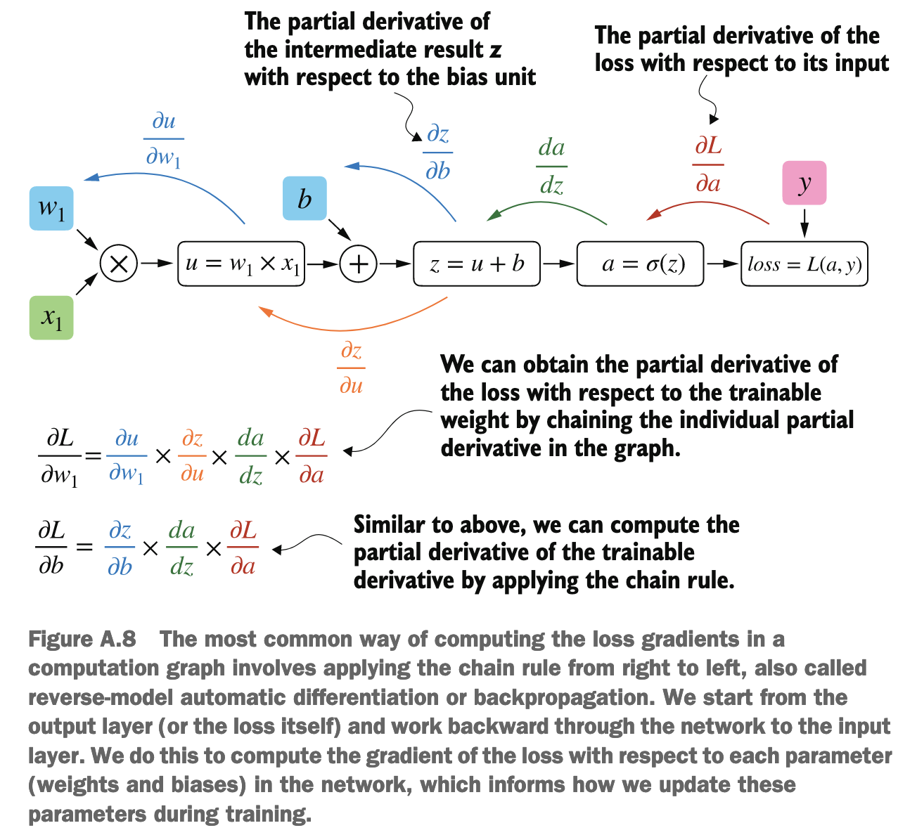
反向传播就可以直接利用上一步的结果进行下一步的计算, 有一点像记忆化搜索
- 多变量函数 (Multivariate function):就是一个有多个输入变量的函数。在深度学习中,损失函数通常是多变量函数,它的输入是模型的所有权重(weights)和偏置(biases)。
- 梯度 (Gradient):梯度是一个向量 (vector)。这个向量的特殊之处在于,它的每一个分量(component)都是该多变量函数相对于其某一个输入变量的偏导数。
如果一个损失函数 取决于很多权重 和偏置 ,那么损失函数 的梯度就是一个包含所有这些偏导数的向量:
这是一个 维的向量
4.2Multilayer Neural Networks#
import torch
import torch.nn as nn

class NeuralNetwork(nn.Module):
    def __init__(self, num_inputs, num_outputs):
        super().__init__()
        self.layers = nn.Sequential(
            # 1st hidden layer
            nn.Linear(num_inputs, 30),
            nn.ReLU(),
            # 2nd hidden layer
            nn.Linear(30, 20),
            nn.ReLU(),
            # Output layer
            nn.Linear(20, num_outputs),
        )

    def forward(self, x):
        logits = self.layers(x)
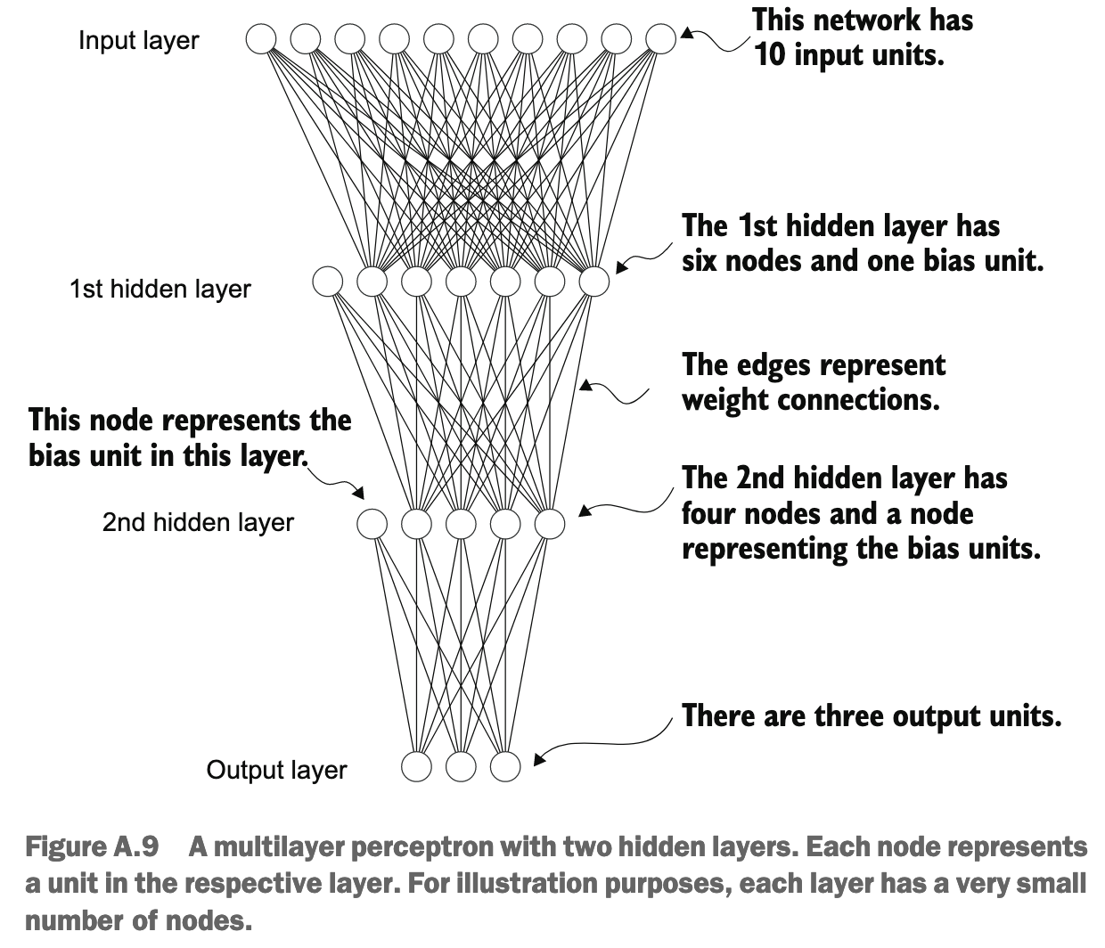
return logitstorch.nn.Linear代表一个全连接层(fully connected layer),这个单元(或层)对其输入执行一个线性变换
执行线性变换:它将输入的 in_features 通过一个权重矩阵 W 和一个偏置向量 b 转换成 out_features。数学表达式为:
其中:
input是输入张量- W 是一个形状为
(out_features, in_features)的权重矩阵。这是该层学习的参数之一。 - b 是一个形状为
(out_features)的偏置向量。这也是该层学习的参数之一 - 表示权重矩阵 W 的转置
分解一下各个部分的维度:
input(输入张量):- 通常,输入是一个批次 (batch) 的数据。如果每个输入样本有
in_features个特征,并且批次大小为batch_size,那么input的形状是(batch_size, in_features)。 - 为了简单起见,我们先考虑单个输入样本,可以看作一个行向量,形状为
(1, in_features)。
- 通常,输入是一个批次 (batch) 的数据。如果每个输入样本有
W(权重矩阵,PyTorch中nn.Linear层的weight参数):- 在 PyTorch 的
nn.Linear(in_features, out_features)层中,其内部存储的权重矩阵self.weight(我们在这里称之为 W)的形状是(out_features, in_features)。 - 这个形状的含义是:它有
out_features行,每一行对应一个输出神经元的权重;它有in_features列,每一列对应一个输入特征的权重
- 在 PyTorch 的
b(偏置向量):- 形状是
(out_features)。在进行加法时,它会被广播(broadcast)以匹配输出的形状。
- 形状是
output(输出张量):- 我们期望的输出形状是
(batch_size, out_features)(或者对于单个样本,是(1, out_features))
- 我们期望的输出形状是
在 PyTorch 中,推荐模型直接输出 logits,然后使用像 torch.nn.CrossEntropyLoss 或 torch.nn.BCEWithLogitsLoss 这样的损失函数。这样做的好处是:
- 代码更简洁:你不需要在模型中显式添加
Softmax或Sigmoid层(除非你确实需要在模型输出概率值用于其他目的,比如在推理时)。 - 训练更稳定:结合的损失函数内部使用了数值技巧来避免计算过程中可能出现的上溢或下溢问题。
- 计算更高效:合并的操作通常经过优化,运行速度更快。
4.3Data Loaders#
import torch
from torch.utils.data import Dataset, DataLoader

class ToyDataset(Dataset):
    def __init__(self, X, y):
        self.features = X
        self.labels = y

    def __getitem__(self, index):
        one_x = self.features[index]
        one_y = self.labels[index]
        return one_x, one_y

    def __len__(self):
        return self.labels.shape[0]


torch.manual_seed(123)

train_loader = DataLoader(
    dataset=train_ds,
    batch_size=2,
    shuffle=True,
    num_workers=0
)

test_loader = DataLoader(
    dataset=test_ds,
    batch_size=2,
    shuffle=False,
    num_workers=0
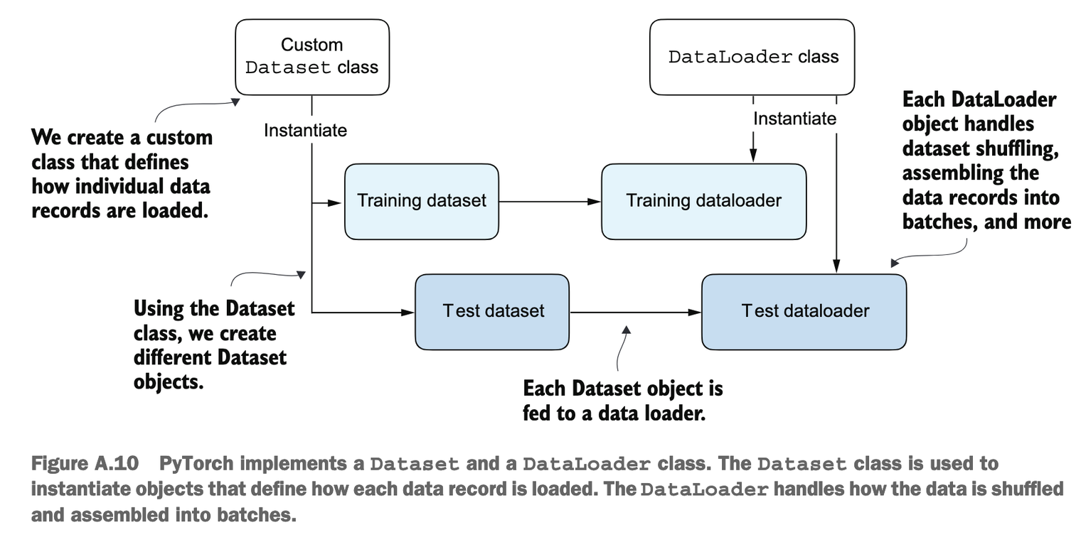
)- 在数据科学和机器学习中,通常约定数组/张量的第一个维度代表样本的数量
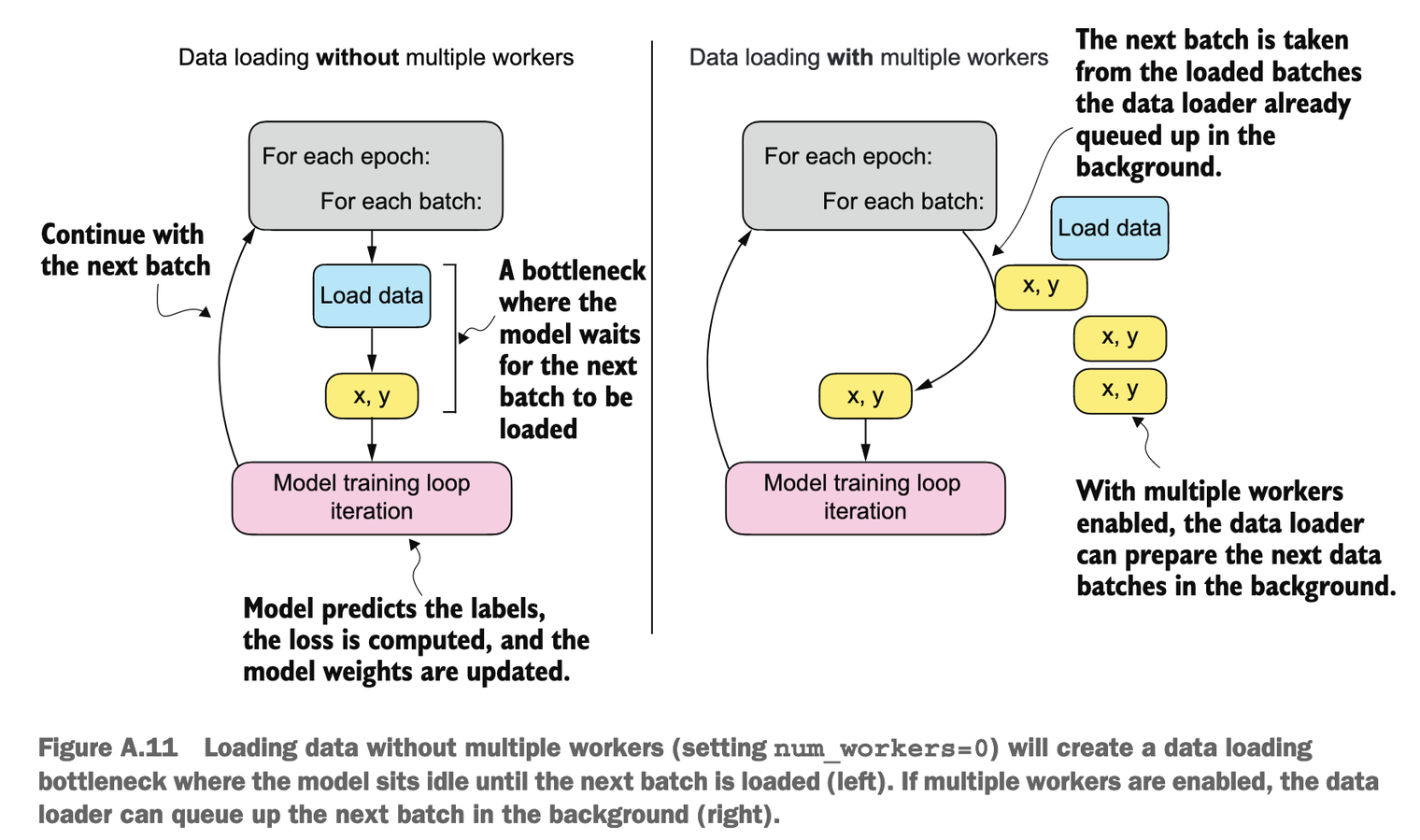
- 当
num_workers被设为 0 时,意味着所有的数据加载操作都将在主进程中串行执行 - 可以加上
drop_last=True来避免不完整的 batch
4.4Training Loop#
import torch.nn.functional as F

torch.manual_seed(123)
model = NeuralNetwork(num_inputs=2, num_outputs=2)
optimizer = torch.optim.SGD(model.parameters(), lr=0.5)

num_epochs = 3

for epoch in range(num_epochs):

    model.train()
    for batch_idx, (features, labels) in enumerate(train_loader):

        logits = model(features)

        loss = F.cross_entropy(logits, labels) # Loss function

        optimizer.zero_grad()
        loss.backward()
        optimizer.step()

        ### LOGGING
        print(f"Epoch: {epoch+1:03d}/{num_epochs:03d}"
              f" | Batch {batch_idx:03d}/{len(train_loader):03d}"
              f" | Train/Val Loss: {loss:.2f}")

    model.eval()
# Optional model evaluationmodel.train()(设置为训练模式)- 作用:此方法告诉模型及其所有子模块(层)它们现在处于“训练模式”。
影响的层:
- Dropout 层:在训练模式下,Dropout 层会按照设定的概率随机地将一些神经元的输出“丢弃”(置为零),这是一种正则化技术,有助于防止模型过拟合。
- Batch Normalization (BatchNorm) 层:在训练模式下,BatchNorm 层会计算当前批次数据的均值和方差,并用它们来归一化数据。同时,它还会更新一个在整个训练过程中持续学习的“运行均值 (running mean)”和“运行方差 (running variance)”。
- 何时使用:在每个 epoch 开始训练数据迭代之前,你应该调用
model.train(),以确保所有对训练敏感的层都以其正确的训练时行为运行。
model.eval()(设置为评估模式)- 作用:此方法告诉模型及其所有子模块(层)它们现在处于“评估模式”(也常用于推理或测试)。
影响的层:
- Dropout 层:在评估模式下,Dropout 层会被禁用。这意味着所有的神经元都会被激活(或者说,它们的输出会按照训练时保留的概率进行缩放),模型会使用其完整的学习能力来进行预测,得到一个确定性的输出。
- Batch Normalization (BatchNorm) 层:在评估模式下,BatchNorm 层不再使用当前批次数据的均值和方差来归一化。相反,它会使用在整个训练过程中学习到的“运行均值”和“运行方差”来进行归一化。这确保了在评估或推理时,模型的输出是确定性的,并且不依赖于当前输入批次的统计特性。
- 何时使用:当你需要评估模型在验证集或测试集上的性能时,或者在部署模型进行实际预测(推理)之前,都应该调用
model.eval()。在你的代码片段中,它被放在了每个 epoch 训练迭代之后,这通常是准备进行验证或记录模型在固定状态下性能的地方。
4.5Saving and Loading Models#
torch.save(model.state_dict(), "model.pth")

model = NeuralNetwork(2, 2) model.load_state_dict(torch.load("model.pth"))