A Survey on Efficient Inference for Large Language Models

General Background

Resources

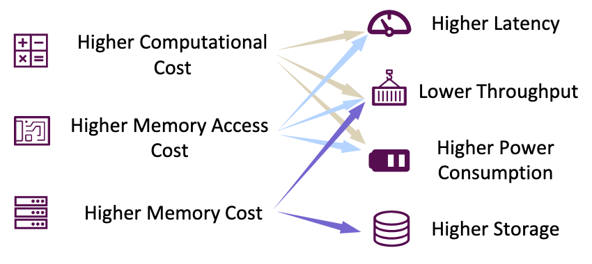
LLMs typically demand:

• Higher Computational Cost
• Higher Memory Access Cost
• Higher Memory Cost

Inference Process of LLMs

auto-regressive generation

In each generation step, the LLM takes as input the whole token sequences, including the input tokens and previously generated tokens, and generates the next token.

With the increase in sequence length, the time cost of the generation process grows rapidly.

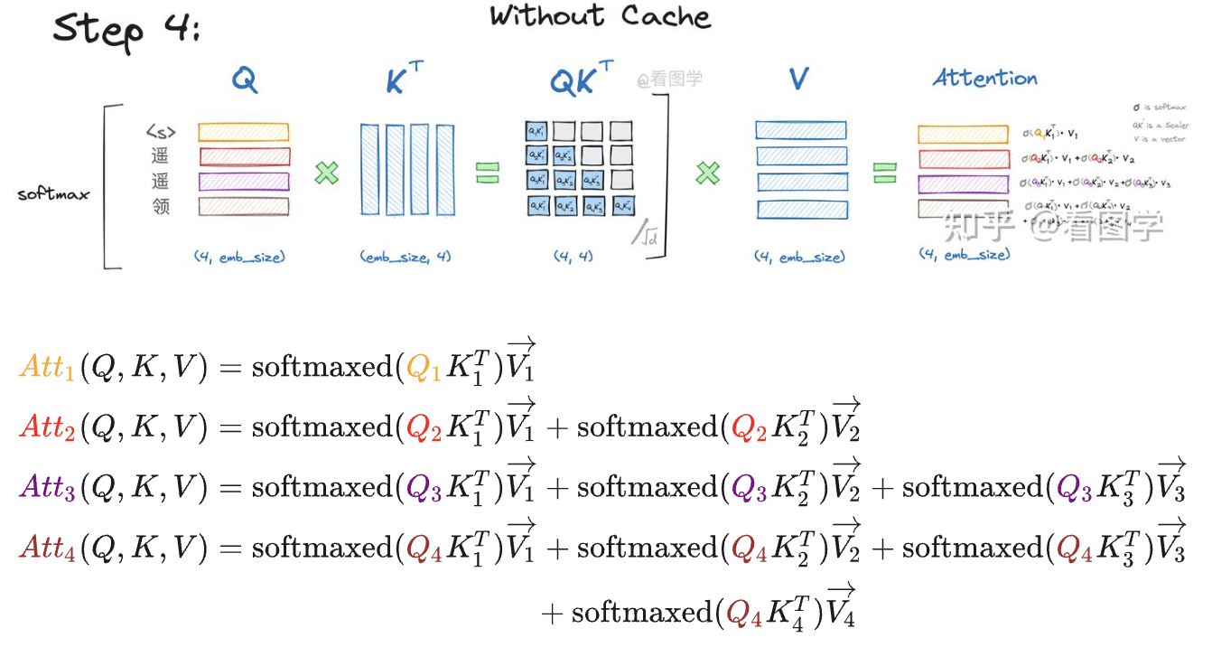
KV cache technique can store and reuse previous key and value pairs within the Multi-Head Self-Attention block.

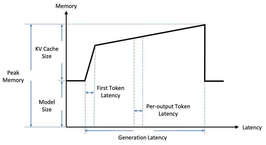
Based on KV cache, the inference process of LLMs can be divided into two phases:

• Prefilling Phase: The LLM calculates and stores the KV cache of the initial input tokens, and generates the first output token.
• Decoding Phase: The LLM generates the output tokens one by one with the KV cache.

Data-level Optimization

Data-level Optimization refers to improving the efficiency via optimizing the input prompts (i.e., input compression) or better organizing the output content (i.e., output organization).

Input Compression

Input compression techniques directly shorten the model input to reduce the inference cost.

• Prompt Pruning: Removing unimportant tokens or sentences from the prompt.
• Prompt Summarization: Compressing a long prompt into a shorter, semantically equivalent summary.
• Soft Prompt-based Compression: Replacing the original long prompt with learnable, shorter continuous vectors (soft prompts).
• Retrieval-Augmented Generation (RAG): Instead of packing all information into the prompt, it retrieves the most relevant information from an external knowledge base to augment it, thereby effectively shortening the context length.

Output Organization

Output organization techniques aim to (partially) parallelize generation via organizing the structure of output content.

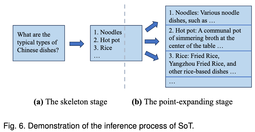
Representative Method: Skeleton-of-Thought (SoT): This method has the LLM first generate a skeleton or outline of the answer, then expands upon and fleshes out each point within the skeleton in parallel, and finally assembles the results into a complete answer. This allows a process that would otherwise require multiple serial decoding steps to be completed in a single batch inference, significantly increasing speed.

Model-level Optimization

The model-level optimization for LLM efficient inference mainly concentrates on optimizing the model structure or data representation.

Efficient Structure Design

direction: right

"Efficient Structure Design" -> "Efficient FFN Design"
"Efficient Structure Design" -> "Efficient Attention Design"
"Efficient Structure Design" -> "Transformer Alternatives"

Efficient FFN Design

The FFN contributes a substantial portion of the model parameters in Transformer-based LLMs: For instance, the FFN module accounts for 63.01% of the parameters in the LLaMA-7B model and 71.69% in the LLaMA-70B model.

Representative Method: It employs the Mixture-of-Experts (MoE) technique, where only a subset of the model’s parameters (the “experts”) is activated for each inference. This allows for an increase in the total number of model parameters while keeping the computational cost of a single inference constant.

In MoE-based Transformers, multiple parallel Feed Forward Networks (FFNs), namely experts, are utilized alongside a trainable routing module. During inference, the model selectively activates specific experts for each token controlled by the routing module.

Efficient Attention Design

• Multi-Query/Group-Query Attention

Multiple attention heads share the same set of Keys and Values, which significantly reduces the memory footprint and access overhead for the KV Cache during the decoding phase.

┌───┐┌───┐┌───┐┌───┐     ┌───┐    ┌───┐             ┌───┐
│ v ││ v ││ v ││ v │     │ v │    │ v │             │ v │
└───┘└───┘└───┘└───┘     └───┘    └───┘             └───┘
│    │    │    │         │        │                 │
┌───┐┌───┐┌───┐┌───┐     ┌───┐    ┌───┐             ┌───┐
│ k ││ k ││ k ││ k │     │ k │    │ k │             │ k │
└───┘└───┘└───┘└───┘     └───┘    └───┘             └───┘
│    │    │    │      ┌──┴──┐  ┌──┴──┐      ┌────┬──┴─┬────┐
┌───┐┌───┐┌───┐┌───┐  ┌───┐┌───┐┌───┐┌───┐  ┌───┐┌───┐┌───┐┌───┐
│ q ││ q ││ q ││ q │  │ q ││ q ││ q ││ q │  │ q ││ q ││ q ││ q │
└───┘└───┘└───┘└───┘  └───┘└───┘└───┘└───┘  └───┘└───┘└───┘└───┘
◀──────────────────▶  ◀──────────────────▶  ◀──────────────────▶
        MHA                    GQA                   MQA
n_kv_heads =4          n_kv_heads=2           n_kv_heads=1

• Low-Complexity Attention

Reducing the complexity of attention from quadratic to linear, for example, through Kernel-based Attention or Low-Rank Attention.

Transformer Alternatives

Model Compression

Model compression encompasses a range of techniques designed to enhance the inference efficiency of a pre-trained model by modifying its data representation (e.g., quantization) or altering its architecture (e.g., sparsification, structural optimization, and dynamic inference).

direction: right

"Model Compression" -> "Quantization"
"Model Compression" -> "Sparsification"
"Model Compression" -> "Structure Optimization"
"Model Compression" -> "Knowledge Distillation"
"Model Compression" -> "Dynamic Inference"

Quantization

Quantization is a widely employed technique that reduces the computational and memory cost of LLMs by converting the models’ weights and activations from high bit-width to low bit-width representations.

TODO: why quantization reduces computational cost?

Two approaches:

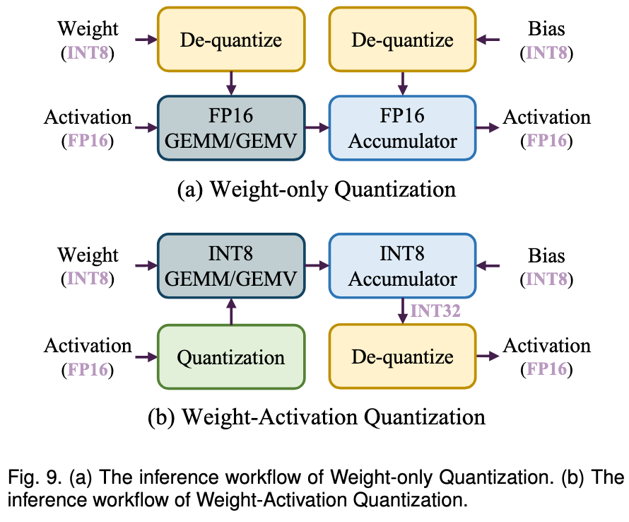
• Weight-Activation Quantization
  • Background:
    • During the prefilling stage, LLMs typically handle long token sequences, and the primary operation is general matrix multiplication (GEMM).
    • The latency of the prefilling stage is primarily constrained by the computation performed by high-precision CUDA Cores.
  • Solution: Quantize both weights and activations to accelerate computation using low-precision Tensor Cores.
• Weight-only Quantization
  • Background:
    • During the decoding stage, LLMs process only one token at each generation step using general matrix-vector multiplication (GEMV) as the core operation.
    • The latency of the decoding stage is mainly influenced by the loading of large weight tensors.
  • Solution: Quantizing only the weights to accelerate memory access.

Post-Training Quantization

Post-training quantization (PTQ) involves quantizing pre-trained models without the need for retraining, which can be a costly process.

Challenge: The weights and activations of LLMs often exhibit more outliers and have a wider distribution range compared to smaller models, making their quantization more challenging.

This foundational approach is simple and fast but can be brittle, especially when dealing with “outliers”—extreme values that stretch the [min, max] range and degrade the precision for the majority of values.

A crucial insight is that different quantization algorithms (like AWQ, GPTQ, SmoothQuant) are not merely choosing different parameters for the same underlying process. Their core innovation lies in the sophisticated pre-processing of weights and activations before the fundamental quantization step is applied.

The goal of advanced quantization algorithms is to perform a pre-processing transformation on the original weights to create a new matrix that satisfies two conditions:

1. Maintains Effectiveness: The new system (e.g., (activation s) (weight / s)) is mathematically or functionally equivalent to the original system before the lossy quantization step.

2. Improves “Quantizability”: The new weight matrix (W_proc) has numerical properties (e.g., smaller dynamic range, fewer outliers) that make it less susceptible to information loss when subjected to uniform, low-bit quantization.

Here are the “philosophies” of different algorithms:

• AWQ (Activation-aware Weight Quantization): “Protecting the Important”

  • Core Idea: Not all weights are created equal. Weights that are multiplied by large, salient activation values are more critical to the model’s performance.

  • Technique: AWQ identifies these important weights and applies a per-channel (which means a row in the matrix) scaling factor. This scaling reparameterizes the weights to protect the most salient channels from significant quantization error, even if it means other, less important weights are quantized less accurately.

• GPTQ (Accurate Post-training Quantization): “Iterative Error Correction”

  • Core Idea: Quantization introduces error. Instead of accepting it, we can actively compensate for it during the process.

  • Technique: GPTQ quantizes weights layer-by-layer and column-by-column. After quantizing one column, it calculates the resulting error and updates the remaining, not-yet-quantized weights in the layer to counteract that error. This iterative correction minimizes the cumulative error across the entire weight matrix.

• SmoothQuant: “Shifting the Difficulty”

  • Core Idea: Activations are often harder to quantize than weights due to their wider dynamic range and more prominent outliers.

  • Technique: SmoothQuant applies a mathematically equivalent transformation. It “smooths” the activations by multiplying them by a scaling factor s (where s < 1) and, to preserve the mathematical output, multiplies the corresponding weights by 1/s. This shifts the quantization difficulty from the activations to the weights, which are more tolerant of it. The result is a system that is easier to quantize with less overall accuracy loss.

Other post-training quantization methods:

See the original paper for full lists.

• OWQ: Employs a mixed-precision strategy by identifying and assigning higher precision to specific weight columns that are associated with activation outliers.
• SpQR: Identifies and allocates higher precision to a small group of weight outliers, while compressing the majority of weights to a very low bit-width.
• SqueezeLLM: Handles outliers by storing them in a separate full-precision sparse matrix and applies non-uniform quantization to the remaining values.
• FineQuant: Uses a heuristic-based approach to determine the optimal quantization granularity for each column in the weight matrix.
• FlexGen: Reduces memory footprint for large batch sizes by quantizing not only the weights but also the KV cache directly into INT4.
• LLM.int8(): Splits the matrix multiplication into two parts, processing channels with activation outliers in high-precision FP16 and the rest in INT8 format.
• RPTQ: Addresses challenging activation distributions by reordering and clustering channels with similar statistics before applying quantization independently to each cluster.

Quantization-Aware Training

Quantization-aware training (QAT) incorporates the influence of quantization within the model training procedure.

Comparative Experiments and Analysis

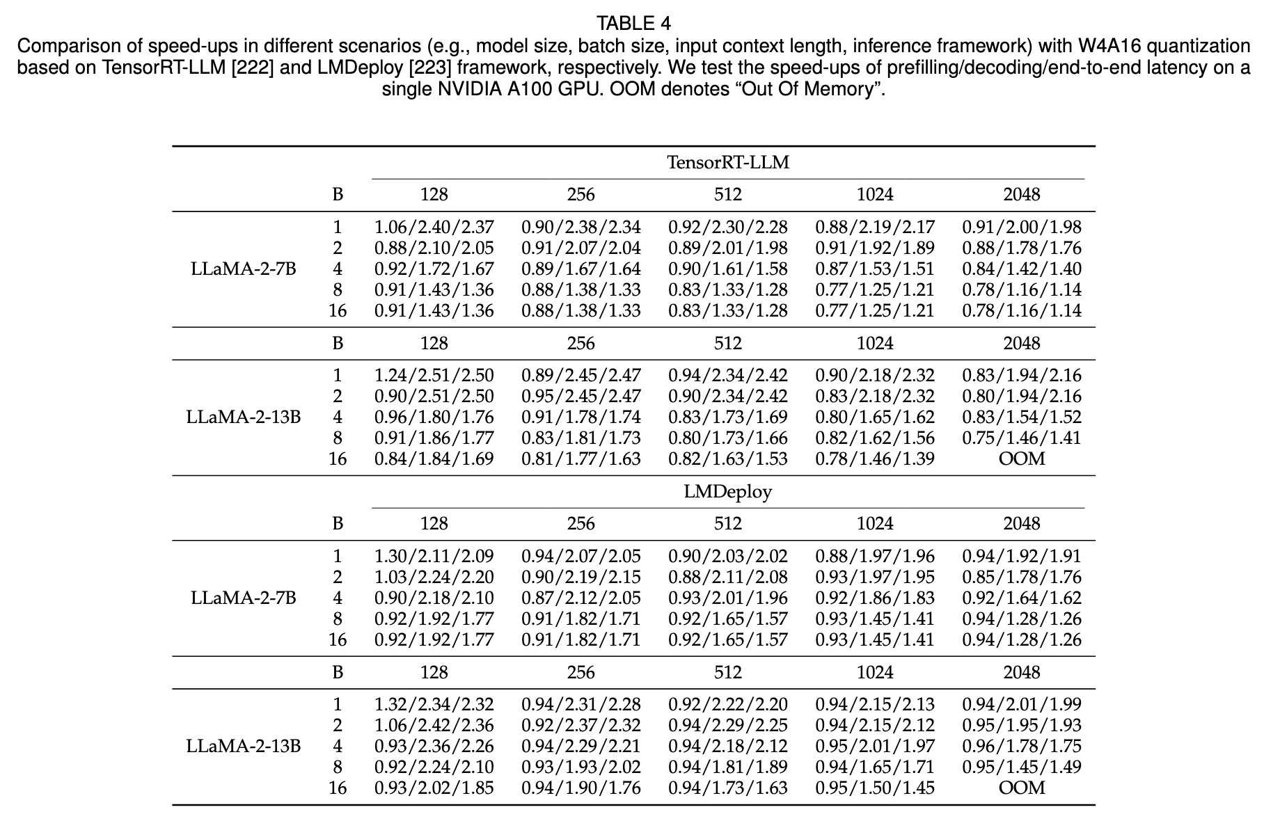
Observations:

• Weight-only quantization can substantially accelerate the decoding stage, leading to improvements in end-to-end latency.
• Regarding the prefilling stage, weight-only quantization may actually increase the latency.
  • The bottleneck in the prefilling stage is the computational cost rather than the memory access cost.
• As the batch size and input length increase, the extent of speed-up achieved by weight-only quantization gradually diminishes.
  • With larger batch sizes and input lengths, the computational cost constitutes a larger proportion of latency.
• Weight-only quantization offers greater benefits for larger models due to the significant memory access overhead associated with larger model sizes.

Sparsification

Sparsification is a compression technique that increases the proportion of zero-valued elements in data structures such as model parameters or activations.

Sparsification aims to decrease computational complexity and memory usage by efficiently ignoring zero elements during computation.

In the context of LLMs, sparsification is commonly applied to weight parameters and attention activations.

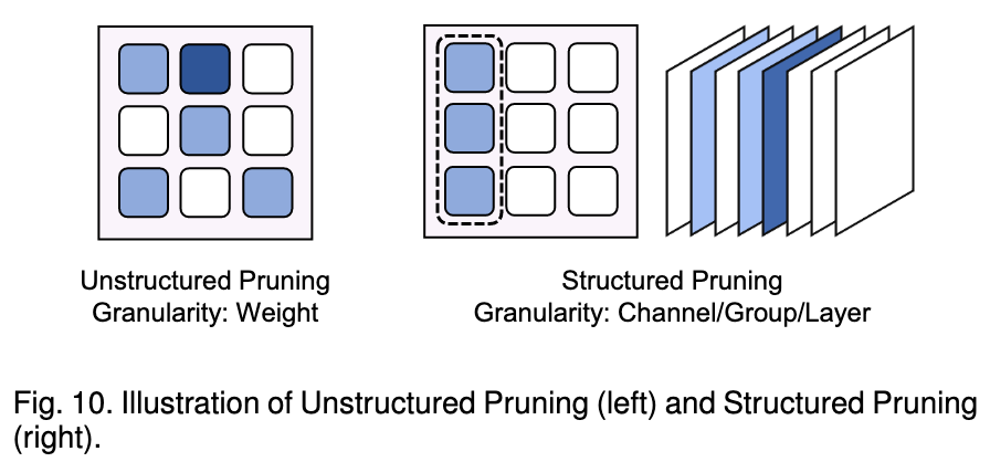
Weight Prune

Weight pruning systematically removes less critical weights and structures from models, aiming to reduce computational and memory cost during both prefilling stages and decoding stages without significantly compromising performance.

It can be categorized into two types:

• Unstructured Pruning: Removes individual, scattered weights. While it can achieve high sparsity with less impact on model accuracy, its irregular pattern makes it difficult to accelerate on modern hardware like GPUs.
• Structured Pruning: Removes larger, regular blocks of the model, such as entire channels or layers. This approach is hardware-friendly and directly leads to inference speed-ups, but it often causes a more significant drop in model performance.

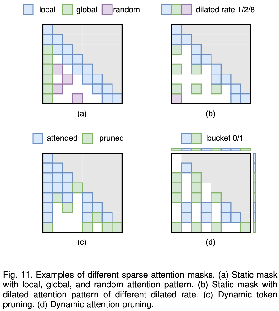
Sparse Attention

Sparse attention techniques in MultiHead Self-Attention (MHSA) components of transformer models strategically omit certain attention calculations to enhance computational efficiency of the attention operation mainly in the prefilling stage.

It also comes in two forms:

• Static Sparse Attention: Uses a fixed, pre-determined sparse pattern that is independent of the input. Common patterns include combining local, global, and random attention to capture different types of information.

• Dynamic Sparse Attention: Adapts the sparsity pattern based on the input data. This can be done by pruning entire uninformative tokens during the generation process or by dynamically clustering related tokens and only computing attention within those clusters.

For detail methods:

Weight Pruning

This method removes less critical weights from the model to reduce its size and computational cost. It is divided into two main types.

Unstructured Pruning

This involves pruning individual, scattered weights within the model. While it can achieve high sparsity with minimal impact on accuracy, it is difficult to accelerate on standard hardware like GPUs due to irregular memory access patterns.

• SparseGPT:
  • Core Idea: It performs one-shot pruning by efficiently calculating the error caused by removing weights and updating the remaining weights to compensate for this loss.
• Wanda:
  • Core Insight: A simple yet effective pruning metric can be created by multiplying the magnitude of a weight by the norm of its corresponding input activation, avoiding complex computations.
• RIA:
  • Core Idea: It prunes weights based on their relative importance and activations, then converts the resulting unstructured sparse pattern into a hardware-friendly N:M structured pattern for real-world speed-ups on GPUs.

Structured Pruning

This involves removing larger, more regular blocks of the model, such as entire channels or layers. This approach is hardware-friendly and directly leads to inference speed-ups, though it may have a more significant impact on model performance.

• LLM-Pruner:
  • Core Idea: Pruning is guided by identifying and removing groups of neurons that are structurally dependent on each other.
• SliceGPT:
  • Core Insight: By leveraging the mathematical properties of the RMSNorm operation, entire rows and columns can be deleted from weight matrices without harming model performance, enabling significant structured pruning.
• LoRAPrune/LoRAShear:
  • Core Idea: These methods are specifically designed for LLMs fine-tuned with LoRA, using the information within the LoRA modules to guide the removal of parts of the original model.

Sparse Attention

This technique enhances the efficiency of the attention operation, mainly during the prefilling stage, by strategically skipping some attention calculations.

Static Sparse Attention

The sparse attention pattern is fixed and does not depend on the input data.

• Longformer/Bigbird:
  • Core Idea: They approximate full attention by combining several fixed patterns: a local sliding-window attention, a global attention to specific tokens, and a random attention pattern.
• StreamingLLM:
  • Core Insight: An LLM can handle infinitely long contexts by maintaining attention only to the very first few tokens (which act as an “attention sink”) and a recent local window of tokens.

Dynamic Sparse Attention The sparse attention pattern is determined adaptively based on the input data.

• Token Pruning (e.g., Spatten):
  • Core Idea: It dynamically identifies and removes unimportant or redundant tokens from the input, so that subsequent layers have a shorter sequence to process.
• Token Clustering (e.g., Reformer):
  • Core Idea: It groups similar query and key tokens into “buckets” using techniques like Locality-Sensitive Hashing (LSH) and only computes attention within each bucket, avoiding the full quadratic computation.
• Heavy-Hitter Oracle (H2O):
  • Core Idea: It combines efficient local attention with dynamic attention to a small, cached set of important “heavy-hitter” tokens from the past, allowing access to crucial long-range context without full computation.

Structure Optimization

The objective of structure optimization is to refine model architecture or structure with the goal of enhancing the balance between model efficiency and performance.

• Neural Architecture Search (NAS)
  • Core Idea: NAS is a technique that automatically searches for the best-performing and most efficient model architecture from a vast number of possibilities.
  • Main Challenge: It is very computationally expensive because it often requires training and evaluating many different architectures. This high cost makes it difficult to apply directly to very large language models (LLMs).
• Low Rank Factorization (LRF)
  • Core Idea: LRF, also known as Low Rank Decomposition, compresses a large weight matrix by approximating it as the product of two much smaller, low-rank matrices.
  • Main Benefit: This method reduces the model’s memory usage and computational cost. For LLM inference, its key advantage is reducing the number of parameters that need to be loaded from memory, which helps to accelerate the decoding speed.
  • Example Approaches: Different algorithms use this core idea in unique ways.
    • ASVD is an “activation-aware” method that scales the weights based on activation data before factorization.
    • SVD-LLM uses a special data whitening technique to find the least impactful parts of the matrix to remove during compression.
    • LoSparse combines LRF with weight pruning for even greater compression.

Knowledge Distillation

Knowledge Distillation (KD) is a well-established technique for model compression, wherein knowledge from large models (referred to as teacher models) is transferred to smaller models (referred to as student models).

In this domain, methods can be categorized into two main types: white-box KD and blackbox KD.

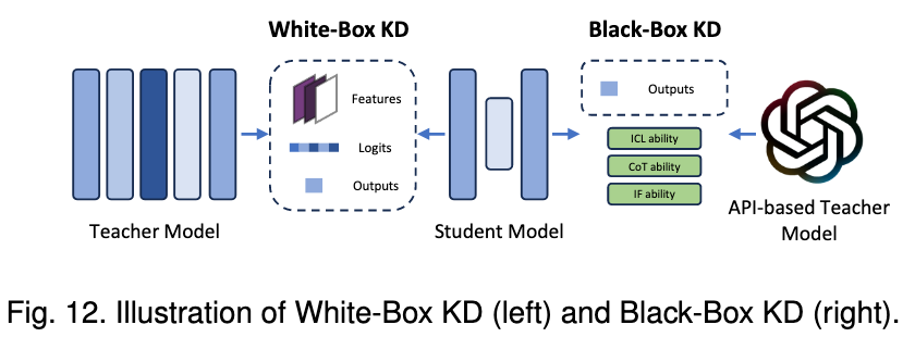
• White-box KD
  • White-box KD refers to distillation methods that leverage access to the structure and parameters of the teacher models.
• Black-box KD
  • Black-box KD refers to the knowledge distillation methods in which the structure and parameters of teacher models are not available.
  • Black-box KD only uses the final results obtained by the teacher models to distill the student models.

Example: deepseek-r1:32b-qwen-distill-q4_K_M

• qwen: The large and powerful teacher model.
• deepseek-r1:32b: The student model. It is a 32-billion parameter model that is smaller and more efficient than the “Qwen” teacher.

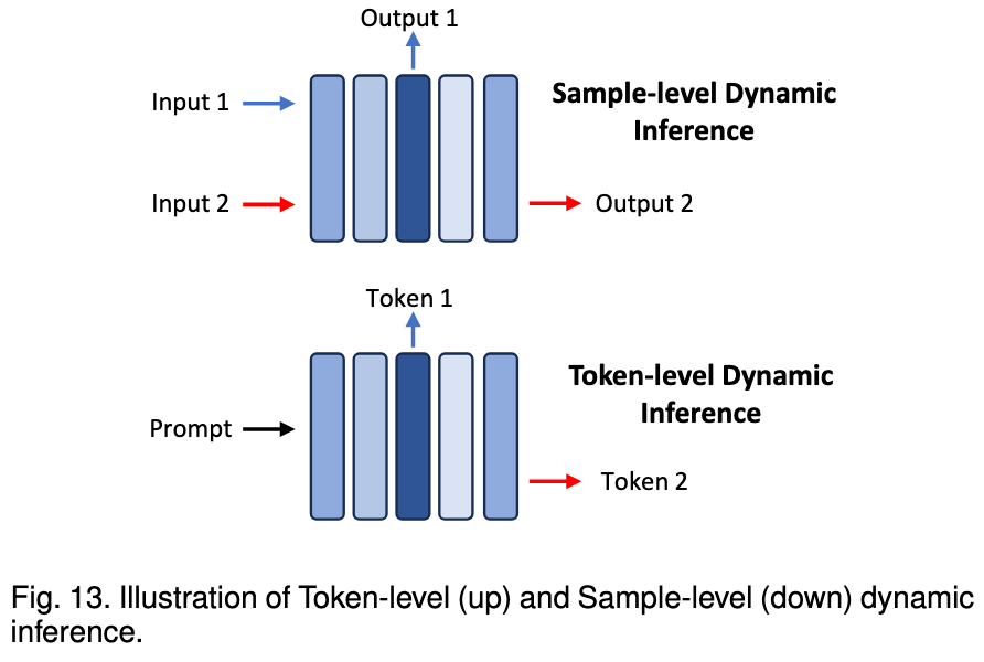
Dynamic Inference

Dynamic inference involves the adaptive selection of model sub-structures during the inference process, conditioned on input data.

This section focuses on early exiting techniques, which enable a LLM to halt its inference at different model layers depending on specific samples or tokens.

The paper categorizes studies on early exiting techniques for LLMs into two main types:

• Sample-level early exiting
  • Sample-level early exiting techniques focus on determining the optimal size and structure of Language Models (LLMs) for individual input samples.
• Token-level early exiting
  • token-level early exiting techniques aim to optimize the size and structure of LLMs for each output token.

System-level Optimization

The system-level optimization for LLM inference primarily involves enhancing the model forward pass.

System-level optimization primarily considers the distinctive characteristics of the attention operator and the decoding approach within LLM.

Inference Engine

The optimizations for inference engines are dedicated to accelerating the model forward process.

direction: right
"Inference Engine" -> "Graph and Operator Optimization"
"Inference Engine" -> "Offloading"
"Inference Engine" -> "Speculative Decoding"

"Graph and Operator Optimization" -> "Attention Operator Optimization"
"Graph and Operator Optimization" -> "Graph-Level Optimization"
"Graph and Operator Optimization" -> "Linear Operator Optimization"

Graph and Operator Optimization

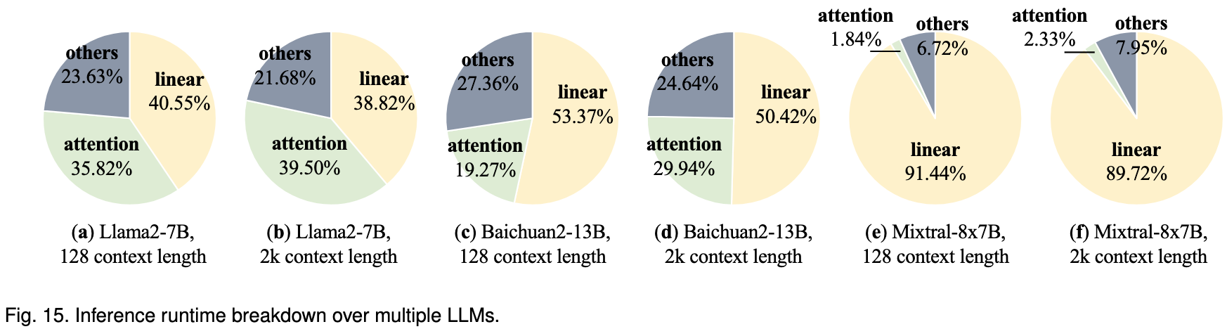
Attention operators and linear operators collectively dominate runtime, with their combined duration often exceeding 75% of the inference duration.

Attention Operator Optimization

The standard attention mechanism is slow and memory-intensive for long sequences.

• Core Idea: The key optimization is to fuse the entire attention calculation into a single, efficient GPU operation, as done by FlashAttention.
• How it Works: Instead of writing the large, intermediate attention matrix to memory, FlashAttention uses tiling to process the calculation in smaller blocks, which significantly reduces memory access and overhead.
• FlashDecoding add more parallelism specifically for the decoding phase.
• FlashDecoding++ further accelerates this by removing synchronization overhead in the softmax calculation.

Linear Operator Optimization

Linear operators (matrix multiplications) are a bottleneck, especially during the decoding stage where they behave like matrix-vector operations, for which standard libraries are inefficient.

• Core Idea: Create custom, highly-optimized kernels for the specific shapes and sizes of linear operations found in LLM inference.
• Solutions:
  • Frameworks like TensorRT-LLM have introduced dedicated General Matrix-Vector Multiplication (GEMV) implementations for the decoding step.
  • For models using Mixture-of-Experts (MoE), MegaBlocks formulates the FFN computation as block-sparse operations and provides custom GPU kernels for acceleration.

Graph-Level Optimization

This involves optimizing the entire sequence of operations, not just individual ones.

• Core Idea: The most common technique is Kernel Fusion, which combines multiple individual operators into a single, larger one.

• Benefits of Fusion:

  • It reduces memory access by eliminating the need to save and load intermediate results between operations.
  • It reduces the overhead of launching many small, separate kernels on the GPU.
  • It can improve parallelism by executing data-independent operations together.

• Examples: Fusing lightweight operations like residual adds and activation functions directly into the preceding linear operator is a common and effective optimization.

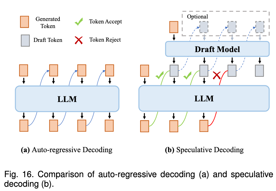
Speculative Decoding

The core idea of this approach involves employing a smaller model, termed a draft model, to predict several subsequent tokens efficiently, followed by validation of these predictions using the target LLM in parallel.

Speculative decoding approach consists of two steps:

1. Draft Construction: It employs the draft model to generate several subsequent tokens.
2. Draft Verification: It employs the target model to compute the conditional probabilities of all the draft tokens in a single LLM inference step, subsequently determining the acceptance of each draft token sequentially.

Offloading

The essence of offloading is to offload part of the storage from the GPU to the CPU when it is free of use.

Serving System

The optimizations for serving systemworks are dedicated to improving the efficiency in handling asynchronous requests. The memory management is optimized to hold more requests, and efficient batching and scheduling strategies are integrated to enhance the system throughput.

Memory Management

The storage of KV cache dominates the memory usage in LLM serving, especially when the context length is long.

• S3 proposes to predict an upper bound of the generation length for each request, in order to reduce the waste of the pre-allocated space.
• vLLM proposes to store the KV cache in a paged manner following the operating system.
• LightLLM treats the KV cache of a token as a unit, so that the generated KV cache always saturates the pre-allocated space.

Continuous Batching

The request lengths in a batch can be different, leading to low utilization when shorter requests are finished and longer requests are still running.

ORCA suggests different requests can be batched at the iteration level.

Core Idea: Instead of waiting for the entire batch to finish, the system checks for completed requests at each step of the generation process (at the iteration level). As soon as a single request finishes, its resources are freed, and a new request from the waiting queue can be immediately added to the batch.

• Chunked Prefill (Split-and-Fuse)

A major challenge is that processing a very long initial prompt (the “prefill” stage) can take a long time and block many other shorter “decoding” requests.

To solve this, frameworks use a method called “split-and-fuse” or “chunked-prefill”.

• How it Works: A long prefill request is broken down into smaller chunks. These smaller prefill chunks are then batched together with the quick, single-token decoding steps from other ongoing requests.
• Benefit: This balances the workload in each batch and prevents a single long request from creating a bottleneck for the entire system, which reduces waiting times (tail latency).

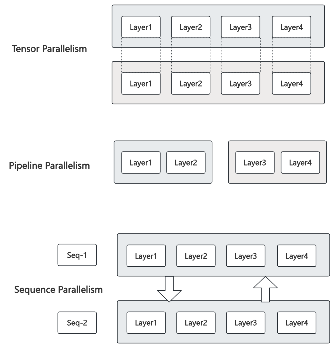
Model Parallelism

• Tensor Model Parallelism (TP)
  • Splits the model layers (e.g., attention, FFN) into multiple pieces from internal dimensions (head, hidden) and deploys each on a separate device (e.g., GPU).
  • Reduce latency through parallel computing.
• Pipeline Model Parallelism (PP)
  • Arranges the model layers in a sequence across multiple devices.
  • Each device is responsible for a pipeline stage that consists of multiple consecutive model layers.
  • Increase the throughput while the latency remains the same.
• Sequence Parallelism (SP)
  • The key idea is to distribute the computational and storage load by splitting the processing of long sequences across multiple GPUs along the sequence length dimension.

Scheduling Strategy

Distributed Systems