EAGLE Speculative Sampling Requires Rethinking Feature Uncertainty
- Doc no.
- KKZ-TN-106
- Date
- 2025-11-10
- GMT day
- 2025:314
- Est. read
- 2 min
Extensive Reading
01Author Info#
02Background#
- The standard method for large language model (LLM) inference, autoregressive decoding, is slow and costly because it generates tokens sequentially, one at a time.
- Existing acceleration methods like speculative sampling often struggle to find a suitable draft model; using a smaller version of the LLM can have high overhead, while training a new, appropriately-sized draft model is prohibitively expensive.
- Other approaches like Lookahead and Medusa successfully reduce drafting latency but are ultimately limited by the low accuracy of their drafts, which restricts their maximum achievable speedup.
03Insights#
Two key insights:
- autoregression at the feature level is simpler than at the token level
- the uncertainty inherent in the sampling process significantly constrains the performance of predicting the next feature
04Approaches#
4.1Preliminaries#
Vanilla autoregression at the token level is described by
for any integer .
- : Tokens
- : Embeddings
- : Features (the output of last transformer layer, or "the second-to-top-layer feature of a LLM, the hidden state before the LM head" in the paper)
- : distributions
解释一下整个过程:
- LLM 输入为一个文字序列,经过 Tokenizer 后成为
- 经过 Embedding 后变为
- 然后经过 Transformer Layers 不断丰富,得到最后包含了对所有内容语义,语法和上下文理解的
- 取最后一个 token 的特征表示
- 通过 LM Head(embedding + softmax) 得到下一个 token 的概率分布 (用 预测 )
- 从 采样得到
Embedding 在两个阶段的数学操作不同:
4.21. 输入阶段:查表(lookup)#
当我们输入一个 token (t_i) 时,它是词表中的一个索引,比如 42。 模型的嵌入矩阵是:
其中:
- (V):词表大小
- (d):embedding(隐藏)维度
查表其实就是选取 (W_E) 的某一行:
这本质上等价于:
也就是说,把 token 变成一个 one-hot 向量,然后乘以整个嵌入矩阵 —— 只是实现上我们用查表来加速而已。
4.32. 输出阶段:矩阵乘法(feature → logits)#
Transformer 最后一层输出一个向量 (), 为了得到每个词的概率(logits),我们要计算:
把特征和所有 embedding 进行相似度计算(点积)
这一步得到一个 (V)-维向量,对应每个词的得分。再经过 softmax:
| 阶段 | 操作 | 数学等价式 | 实现形式 |
|---|---|---|---|
| 输入 | one-hot → embedding | 查表 | |
| 输出 | embedding → logits | 矩阵乘法 |
4.4Feature-level prediction#
利用模型次顶层特征进行自回归预测比直接预测下一个 Token 更简单、更具规律性
- 直接预测 Token ❌
- 直接预测 Feature ✅
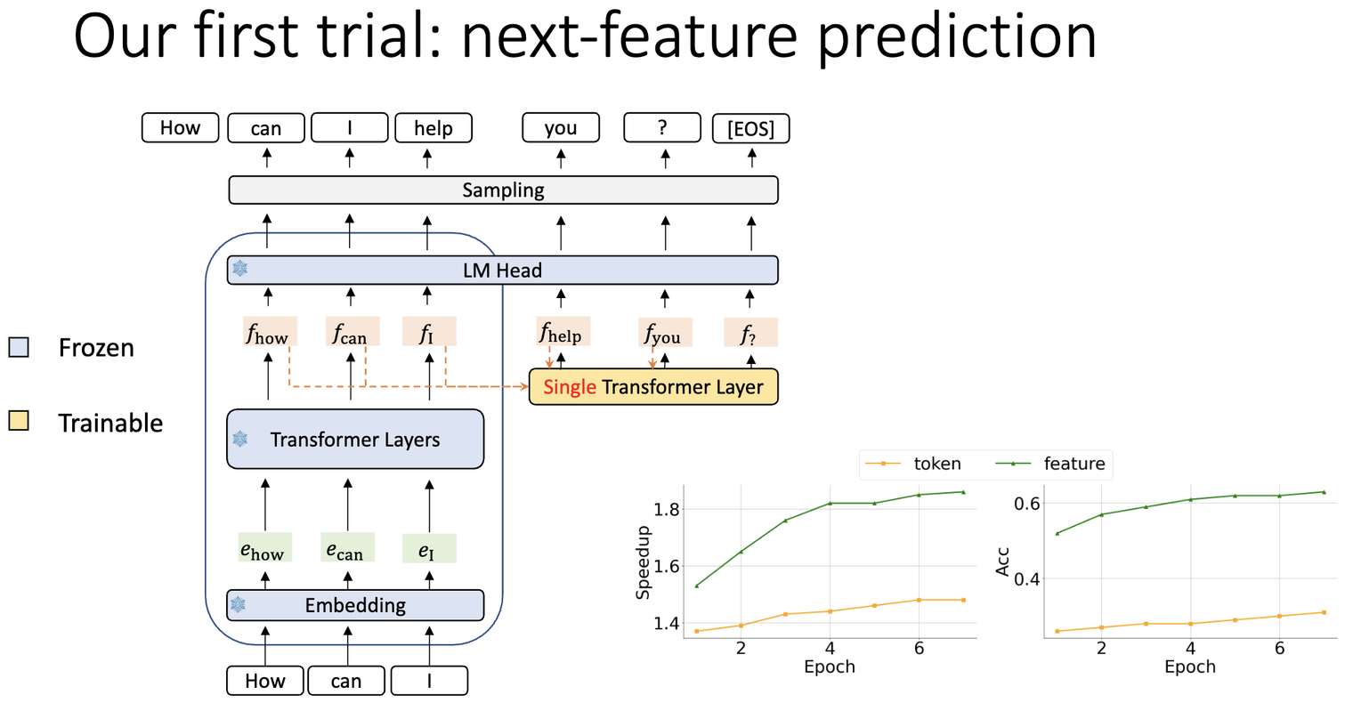
非常 Reasonable:
- 包括了大量的“知识”(语义语法上下文),而采样后的 丢失了这种信息
4.5Feature uncertainty#
如果只用 来进行预测,会出现一个问题:
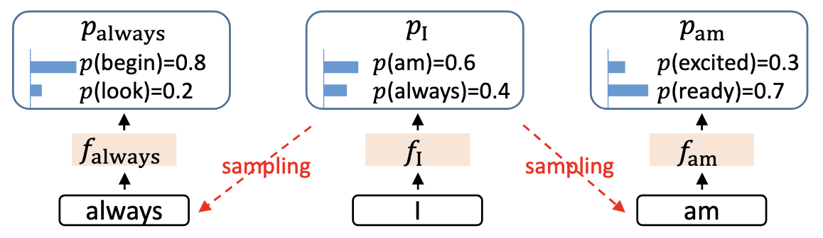
比如上图中, 其实包含了两种采样结果: 和 ,在采样时选择不同的 token 会通向不同的特征 or
在通过 预测 时,我们只希望 中包含一个确定的
Idea: feature & shifted-token -> next feature
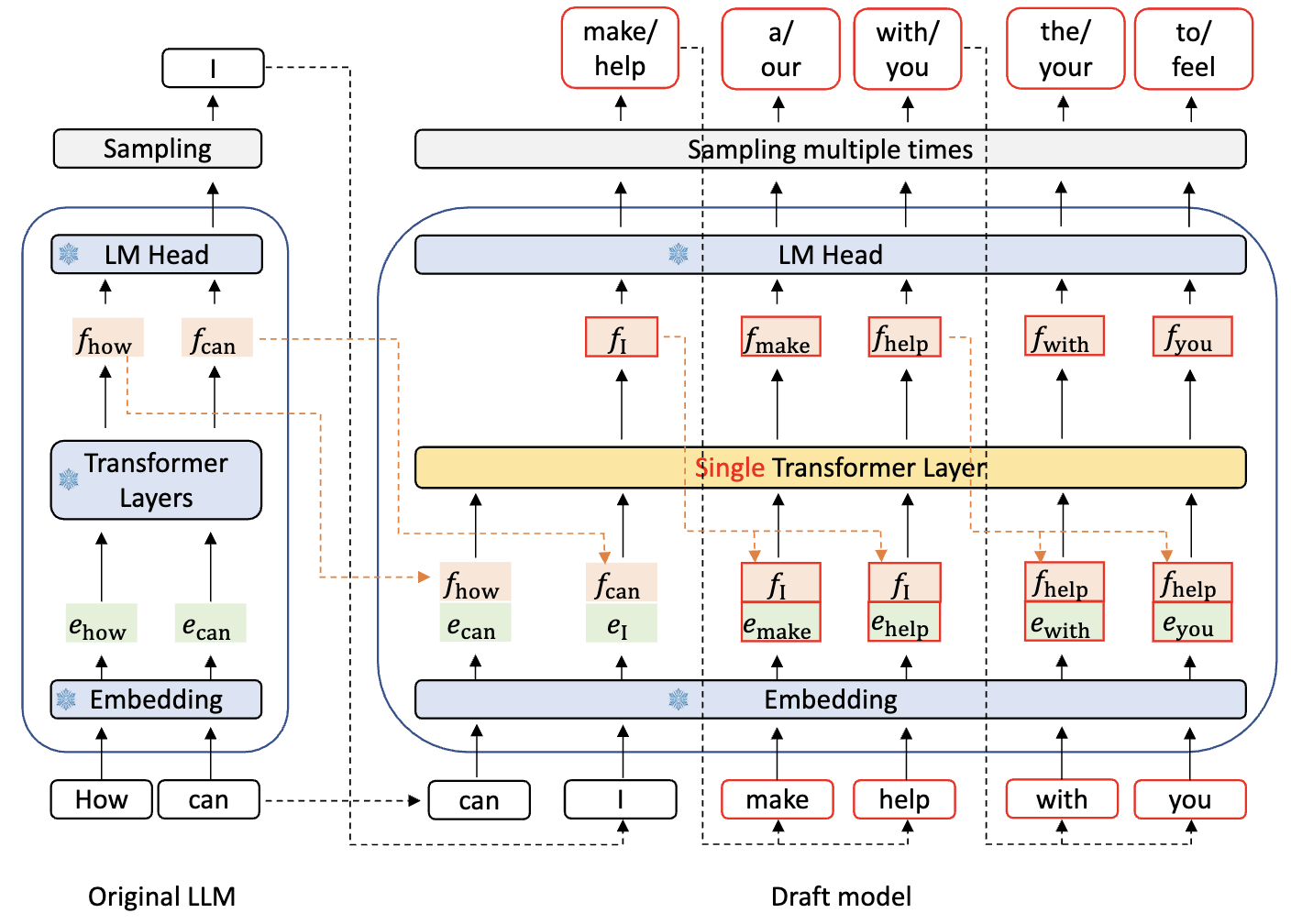
伪代码:
python
# 已知:上一时刻真特征 f_i(来自目标模型某层的隐藏态)
# 步骤:
# 1) 先用 f_i 的 LM Head 采样出 t_{i+1}
logits_i = lm_head(f_i)                     # 复用目标模型 LM Head
t_next = sample_from_logits(logits_i)       # 采样(或取 top-k/温度采样)

# 2) 把 tokens_right_shifted 更新到包含 t_{i+1},喂 AR-Head 预测 \hat f_{i+1}
#    feats_hist 包含到 i 的特征序列;tokens_shifted 包含 t2..t_{i+1}
f_next_hat = ar_head(feats_hist, tokens_shifted, return_all=False)  # [B, H]

# 3) 再用 \hat f_{i+1} 走 LM Head 得到下一步分布,继续采样 t_{i+2}
logits_next = lm_head(f_next_hat)
t_next2 = sample_from_logits(logits_next)

# (可扩展为树:对 t_{i+1} 取多分支并行各自预测 \hat f_{i+1}^{(branch)})4.6Overall Comparison#
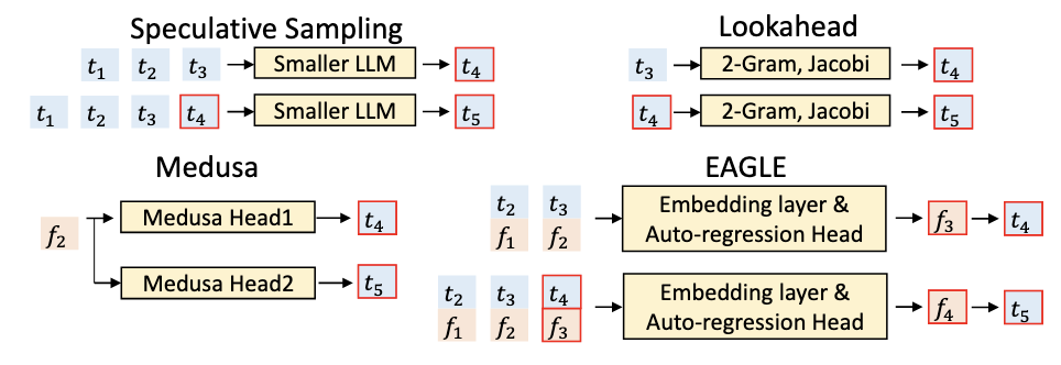
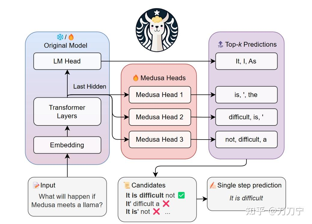
By the way, Medusa overview:
05Evaluation#
06Thoughts#
6.1When Reading#
07Related Works#
Comments