STI Turbocharge NLP Inference at the Edge via Elastic Pipelining

Intensive Reading

Author Info

• Homepage - Liwei Guo / Assistant Professor: a tenure-track Assistant Professor at University of UESTC.

Background

Challenges

• Cold start of NLP models in mobile devices
• NLP inference stresses mobile devices on two aspects
  • Latency: impromptu user engagements
  • Model Size

Existing Paradigms:

• Hold in memory
  • Too large memory footprint, likely to be victims of mobile memory management
• Load before execute
  • Slow start, waiting for I/O, computation resources stall
• Pipeline load/execution
  • Low arithmetic intensity in Transformer’s attention modules
  • The pipeline is filled with bubbles and the computation stalls most of the time at each model layer

Insights

A model can be re-engineered from a monolithic block into a collection of resource-elastic “shards” by uniquely combining vertical partitioning with fine-grained, per-shard quantization. This transforms the I/O time of each model component into a tunable parameter.

A stall-free, optimal pipeline is achievable through a two-stage planner that uses an “Accumulated IO Budget” (AIB) to manage time resources. This allows the system to intelligently spend its limited I/O budget on loading higher-fidelity versions of the most accuracy-critical shards, thereby maximizing performance under strict latency constraints.

Approaches

Elastic Model Sharding

为了让模型能够灵活适应不同的资源约束，STI 首先对预训练好的模型进行预处理，将其分解为大量可供运行时选择组合的“分片”（Shards）。这个过程分两步:

• Step 1: 垂直分区
  • 将 Transformer 的每一层（N层）沿着宽度方向，切分为 M 个垂直切片（vertical slices）,每个切片包含一个独立的注意力头以及对应比例的 FFN 神经元
• Step 2: 分片量化
  • 针对每一个 sharding，STI 会为其生成 K 个不同量化的版本
  • 采用高斯离群点感知量化方法, 将绝大多数遵循高斯分布的权重用 k-bit 索引指向一个小的“质心”字典来表示，而保留极少数重要的离群点权重为 32-bit 浮点数

在大模型中仍然适用吗？

通过以上两步，一个N层的模型被预处理成了磁盘上的 N x M x K 个分片版本，为运行时的弹性规划提供了丰富的选择空间。

Pipeline Planning

这部分主要是通过一定的定量分析给出了一个数学建模，然后在此基础上来确定计划的构建，分为两步

1. 根据 Client 给出的总时间预算 T, STI 确定需要计算的 submodule 大小（n x m），目标是 n x m 的计算量越大越好（接近上限）
2. 根据 n x m，STI 再去算对应的 AIB, 然后确定每个 shard 使用什么量化（根据量化重要程度排序），目标是 让 AIB >0 的同时精度也更高

• 确定量化时使用了一个 two-pass 的分配策略
• First Pass: 首先为所有需要动态加载的分片选择一个统一的、在不违反AIB约束下的最高基础位宽
• Second Pass: 然后利用剩余的AIB预算，根据分片重要性排名，贪婪地、迭代地将最重要的分片升级到更高的位宽（最高可达32-bit），直到所有AIB预算被耗尽

AIB: Accumulated IO Budgets

核心思想：

流水线不会停顿的充要条件是：在执行第 k 层的计算之前，从第 0 层到第 k 层的所有分片都必须已经被加载到内存中 。基于这一点，AIB 被设计为一个记录“可用 IO 时间余额”的账本。在计算前面层的时候，IO 设备是空闲的，这段计算时间就可以被“存入” AIB，作为加载后续层数据的“预算”。

$AIB(k) = AIB(k-1)+T_{comp}(k-1)$

• $AIB(k-1)$: 上一层累积下来的 IO 预算
• $T_{comp}(k-1)$: 计算第 k-1 层所需的时间

只要所有层的 AIB 值都 大于等于零，就意味着在任何一层开始计算之前，它所需要的数据都能及时加载完毕，流水线不会停顿，因此该规划方案被视为有效

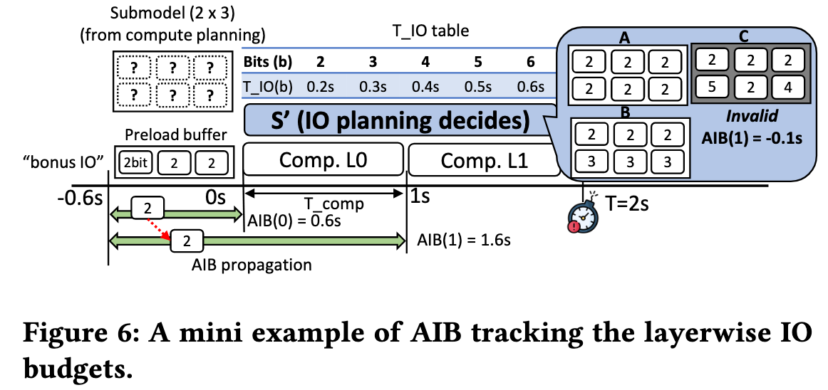
以图 6 举个例子：

• 计算规划阶段已经完成，确定了要运行一个 2层 x 3分片 的子模型
• 总任务耗时不能超过 T = 2s， T_comp = 1s
• L0 预加载了第 0 层的 3 个分片，都是 2-bit 版本
• AIB(1)=1.6s: 在第1层（L1）的计算开始之前（即在 t=1s 这个时间点），我们总共有 1.6 秒的时间可以用来加载所有需要的数据
• 留给 L1 的预算是 1.0s

Evaluation

Thoughts

When Reading

能否针对 one-shot 和 interactive 场景做不同优化？

“Sparsity is all you need”:

• Attention heads can be predicted
• Experts in MoE can be predicted
• FFN block which passes the gate can be predicted

Predict-and-prefetch is all you need

不适合目前的大模型：

• 存储开销：每个 shard 要存 {2,3,4,5,6,32} 共 6 个版本，虽然作者称只需 ~215MB 额外存储 (Sec.7.2)，但对于大模型（>10B 参数）存储成本将线性放大
• Profiling 的开销也会爆炸

Related Works

• EdgeMoE Empowering Sparse Large Language Models on Mobile Devices
• LLM as a System Service on Mobile Devices